The study was designed as a natural experiment, since we assume that urgency level is unassociated with traffic conditions and considered random. We collected observed transport times for ambulances dispatched with urgency Level A and B from March 10 to June 11, 2021, and compared them with their corresponding estimated transport times. The estimated transport times were conditioned on corresponding weekday, time-off-day, weather conditions, and major changes to road network within 3 weeks of the observed transportation. No larger lockdowns due to the COVID-19 pandemic were started or ended within the inclusion period.

Patient transports were included if departing by ambulance on land from private addresses throughout the Central Denmark Region and arriving at one of the region’s six EDs.

The study was conducted in the Central Denmark Region, one of the five Danish regions, with a size of 13.011 km2 and a total population of 1.38 million [17, 18]. The demography of the area is mixed urban and rural with a total population density of 100.3 people per km2 with a span from 717.5 people per km2 in the biggest city of the region (Aarhus), to 8–35 people per km2 in rural areas [19, 20].

In the Central Denmark Region, the emergency calls from citizens are received and managed by one central Emergency Medical Dispatch Center (EMDC). Based on the symptom, believed to be most important, the EMS dispatcher allocates resources (e.g., an ambulance with or without a physician manned rapid response vehicle and/or helicopter) and determines the level of urgency using The Danish Index (DI). DI is a criteria-based dispatch protocol that consists of 37 main symptom groups (organized in chapters). Each chapter is subdivided into five levels of urgency. Three levels are dispatched for patients in need of medical treatment: Level A for life-threatening or potentially life-threatening conditions, requiring an immediate response dispatched during the emergency call conversation; Level B for urgent, but not life-threatening conditions dispatched within 30 min from the emergency call; and Level C for transport less urgent that should be dispatched within 1–2 h after the emergency call (mostly used for inter-hospital transfers and general practitioner arranged transports). Only Level A transportations uses L&S and are allowed to break traffic rules, e.g., exceeding posted speed limits, proceeding through red traffic signals, stop lights or stop signs, bypassing traffic jam, and using alternative routes, e.g., sidewalk etc. Each emergency call is assigned a DI criteria code that corresponds to the level of emergency, based on the main symptom and a specific subgroup symptom. At scene, the EMS providers assess the patient and decide whether the patient should be transported to the nearest acute medical department or specialized care. However, before departure from the scene, the EMS providers inform the receiving department, and a second opinion may be utilized. In various scenarios, ambulances may bypass nearby EDs, proceeding directly to specialized departments. For instance, local ED bypass is frequently observed in Level A transports involving patients suspected of stroke or acute myocardial infarction. Similarly, patients transported by Level B urgencies may also bypass local EDs, particularly under open admission agreements for cancer patients.

In cases where patients exhibit highly unstable vital signs, the ambulance often prioritizes proximity and heads directly to the nearest acute medical department, setting aside the bypass strategy. Consequently, the cumulative distances covered in Level A or B transports can vary based on the specific circumstances and the urgency of the medical condition.

Simultaneously, the level of urgency initially decided by the EMS dispatcher can be down or upgraded. Level of urgency from the scene to hospital can, therefore, differ from the initial dispatched urgency level.

In this study, dispatched Level A driven as Level A to hospital is noted A–A, dispatched Level A downgraded at scene and driven as Level B as A–B, and dispatched Level B driven as Level B as B–B. Transports dispatched as Level B driven as Level A were limited and could not form an independent group, thus, excluded.

Data from the EMDC dispatch system (Logis) and the electronic Prehospital Patients Record (ePPR) included addresses and coordinates of the scene of the accident/incident and the receiving hospital; time and date of the departure from scene and arrival at hospital; total transport duration; the Logis system’s ETA; the DI dispatch code (containing the dispatched level of urgency); and the level of urgency of the ambulance transport to hospital.

The Google Maps Application Programming Interface (API) was assessable for public use. Google Maps Distance Matrix API was used to make requests from Google Maps on the estimated transport times both non-traffic and traffic adjusted. To retrieve Google Maps estimates, we used R [R Core Team (2022). R: A language and environment for statistical computing. R Foundation for Statistical Computing, Vienna, Austria. URL https://www.R-project.org/] [21].

Addresses of all scenes of incident and receiving hospitals were converted to latitude and longitude coordinates from ePPR to provide estimated transport times in the Google Maps system. It is not possible to get estimates of historical transports in Google Maps, and thus, the corresponding estimation of duration for each transport were retrieved within 3 weeks after the transport took place conditioned on corresponding weekday, time-off-day, weather conditions, major changes to road network (e.g., road network changes, major events creating a traffic jam, etc.).

Departure time was grouped according to morning rush hour (07:00–09:00), daytime (09:00–15:00), afternoon rush hour (15:00–17:00), and nighttime (17:00–07:00). The mode was set to ‘driving’ and traffic-model was set to ‘best guess’, which was the best estimate of travel time given what was known about both historical traffic conditions and live traffic information.

We retrieved data on the daily weather conditions from the Danish Meteorological Institute (DMI). Weather conditions were only grouped according to above or below 2 ℃. However, transports that took place on days with reports of snow, heavy rain (defined as more than 24 mm within 6 h), and heavy fog (defined as visibility less than 100 m) were excluded. Transportations where it was impossible to find an estimated transportation duration corresponding to the stated conditions were also excluded.

The outcome was transport duration from scene of accident to receiving hospital department.

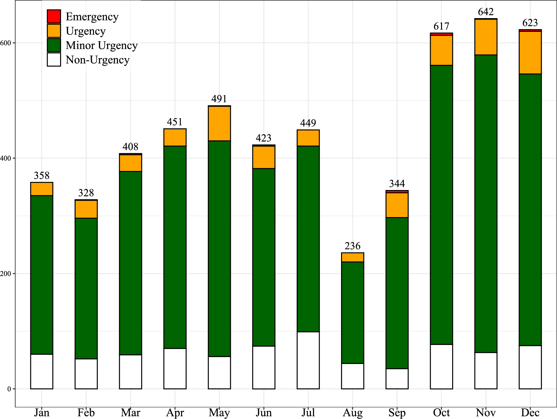
Initially, we summarized the distribution of urgency level among indications for emergency transport using the DI. Distributions were presented as frequencies and percentages, and indications of emergency transports which represented less than 100 transports were discarded.

In the primary analysis, we estimated absolute and relative differences in medians between observed and estimated transport durations. These were stratified by Level A–A, A–B, and B–B. Results were calculated as duration of the entire transport and per 10 km. Standard errors were estimated using bootstrap with 1000 replications. In addition, results were stratified by distances below 10 km, from 10 to 20 km, and above 20 km.

We conducted a sensitivity analysis where we used the estimated transport times provided by Logis instead of Google maps.

Finally, using restricted cubic splines, we conducted median regression spline curve analysis on transports less than 100 km to visualize duration as a function of distance comparing Level A–A and B–B transports with Google Maps estimated durations. From the spline curves, we were able to estimate the median delay from the ambulance personnel activated Logis and until the ambulance left the scene. This delay was estimated by subtracting the intercept of the spline curves for the observed transport durations with the intercept of the spline curves for the estimated durations.

Results were presented with 95% confidence intervals (CI) and data were analyzed using Stata 17 (StataCorp. 2021. Stata Statistical Software: Release 17. College Station, TX: StataCorp LLC.).