Corpus

A typical research article usually consists of five sections: introduction, methodology, results, discussion, and conclusion. The abstract is the summarization of the research, including such key rhetorical moves as introduction, purpose, method, results and conclusion (Hyland, 2000). To summarize the whole article in a limited space, the article writer is impelled to compose a text with “maximum efficiency, clarity and economy” (Swales and Feak, 2009). As noted by Biber and Gray (2011), NGs contribute significantly to the compressed style of writing commonly observed in abstracts. Gray (2015) pointed out that abstracts showed the densest use of phrasal features, which serve as a strong indicator of NG complexity (Gray, 2013). Furthermore, full sentences are used in abstracts with no inserted non-linguistic information such as figures and tables. This is reliable for calculating clause constituents.

Abstracts exhibit distinct linguistic characteristics across disciplines (Hyland, 2000). In natural sciences (e.g., medicine, physics, and computer science), abstracts tend to use passive voice, emphasizing research methods and results while minimizing subjectivity (Pho, 2008). In contrast, abstracts in social sciences (e.g., linguistics, education, and management) often employ active voice, highlighting the research background and significance (Lores, 2004). Humanities abstracts, on the other hand, often incorporate more evaluative language, emphasizing the theoretical contributions of the research (Hyland and Tse, 2005). Given the varying organizational patterns, the linguistic resources influencing the DD in academic writing may similarly vary across disciplines, shaped by disciplinary norms.

This study is based on a self-built corpus of 1,050 research article abstracts, collected from research articles published between 2017 and 2022 in the Web of Science database. In selecting abstracts for this study, we adhered to the fundamental classification of disciplines into hard and soft sciences as outlined by Biglan (1973). Recognizing that this broad categorization may overlook the unique linguistic features of individual disciplines, we further subdivided soft sciences into Humanities and Social Sciences (SS). This approach resulted in three major disciplinary groups: Humanities (e.g., Literature and History), Social Sciences (e.g., Business and Politics), and Natural Sciences (e.g., Physics and Biology).

To enhance the representativeness of the self-built corpus, we also considered the Journal Citation Indicator (JCI), a metric that evaluates journal performance in Web of Science. Due to the variation of JCI values across disciplines, we balanced the JCI values by restricting the JCI range within each discipline. See Table 1 for a detailed breakdown.

Table 1 Descriptive statistics of the corpus.Data collection

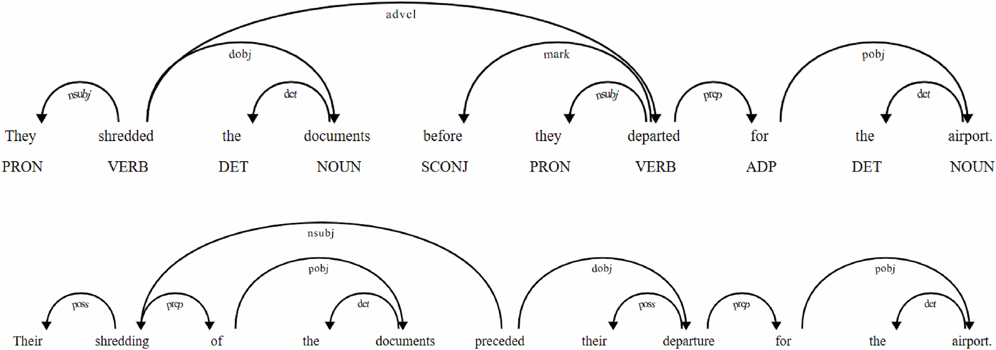
The corpus was converted into dependency-annotated treebanks for each sentence using SpaCy (Honnibal and Montani, 2019) in Python. A custom Python script was written to analyze the dependency relations within each sentence in the corpus. The corpus texts were first segmented into sentences. Within each sentence, the root HVs and their governed HVs correspond to the number of clauses. Furthermore, in any given clause, the number of HNs governed by an HV directly reflects the number of participant NGs. Example (5) demonstrates the calculation of the DD between the HV and the subject HN, as well as between the HV and the object NG.

(5)

This article discusses the largely forgotten antiwhaling protests in Norway and Japan at the beginning of the twentieth century. (Humanities)

The DD between the HV discusses and the subject HN article is 1, and that between the HV discusses and the first premodifier of the object NG the largely forgotten anti-whaling protests is also 1. Within the NG, the DD between the subject HN article and the determiner this is 1, and the DD between the object HN protests and the determiner the is 4.

In total, we collected 21,246 participant NGs, including 8497 in SS texts, 6111 in Humanities texts, and 6638 in NS texts. See Table 2.

Table 2 Participant NGs in the corpus.

However, the DD between the HV and the subject HN does not necessarily reflect clause complexity, as it may be influenced by the presence of post-modifiers of the HN. For example:

(6)

a. Impending abolition of slavery in Brazil during the late nineteenth century meant the potential shortage of labor for Southeast coffee planters. (Humanities)

b. A sharp and statistically significant increase in SRB appears with the war. (Humanities)

Both (6a) and (6b) consist of three clause constituents, and hence they exhibit the same clause complexity. The DD between the HV meant and the subject HN abolition is 10 in (6a), whereas the DD between the HV appears and the subject HN increase is 3 in (6b). However, the three prepositional phrases of slavery, in Brazil and during the late nineteenth century in (6a) and the one prepositional phrase in SRB in (6b) are the rank-shifted use of phrases within NGs, functioning as post-modifiers of the HNs in the NGs. These phrases have their own syntactic structures, and so it would be inappropriate to include them in the calculation of the lengths of the NGs.

In the present study, we considered only the premodifiers of the HN as contributing to the complexity of the NG. From this perspective, the DD between the first premodifier impending and the subject HN abolition is 1 in (6a), whereas the DD between the first premodifier a and the subject HN increase is 5 in (6b), indicating that the subject NG in (6b) is more complex than that in (6a).

Data analysis

In our analysis, we employed the independent t-test in SPSS 29 to compare the mean DDs between different disciplinary groups and to determine whether the differences were statistically significant. When the variances of the two groups were unequal, we utilized Welch’s t-test. The formula for the t-test statistic is as follows:

$$t=\frac}_-}_}_^}_}+\frac_^}_}}}$$

where \(}_\) and \(}_\) represent the means of the two groups, \(_^\) and \(_^\) are the sample variances of the two groups, and \(_\) and \(_\) are the sample sizes of the two groups. We set the significance level at 0.05 for the critical t-value. A significant difference between the two groups is indicated if the t-value exceeds the critical t-value or if p < 0.05. It should be noted that we used the independent t-test to compare the mean differences between the data groups. The result, however, might be affected by the extreme values, and so boxplots were employed to identify and address the potential outliers in the dataset.

Additionally, we investigated the relationship between the DD and its frequency using the Menzerath–Altmann Law (Altmann, 1980), which is mathematically modeled by the following formula:

where the variable x represents the size of the whole unit, and y represents the average size of the subunits. In this study, x denotes the DD, and y represents the corresponding frequency.

This function integrates a power law and an exponential decay. When x is small, the power law \(y=a^\) predominates, which controls the initial growth or decay rate of the function. As x increases, the exponential decay takes over, which causes the function to decay rapidly and approach zero. Parameter a in the function is a scaling constant that sets the initial value or height of the curve on the y-axis. Parameter b influences the initial rate of growth or decay. If b > 0, the curve initially stretches upward rapidly as x increases. A larger b results in a faster increase in y as x grows. Conversely, if b < 0, the curve decreases rapidly as x grows. If b = 0, the function behaves as a pure exponential decay. Parameter c controls the rate of exponential decay. A larger c indicates a faster decay, while a smaller c results in a slower decay.

We also employed Pearson’s Chi-squared test in SPSS to analyze the distribution of the data across disciplinary groups and determine whether the differences were statistically significant. The formulas for conducting Pearson’s Chi-squared test are as follows:

$$^=\sum \frac_}-_})}^}_}}$$

where \(_}\) represents the observed frequency in each category, and \(_}\) is the expected frequency for each category. The indices i and j correspond to the rows and columns, respectively, in the contingency table, while n is the total number of observations. A significant difference between the two variables is indicated if the \(^\) value exceeds the critical value or if p < 0.05.