A realistic finite element method (FEM) model of the thorax was constructed based on anatomical data from the lower thoracic spinal level (T11) [23] and surrounding anatomical tissues [24, 25]. The model was segmented into 12 tissues, including skin, fat, muscle, general thorax, bone, vertebrae, intervertebral disks, extradural tissue, dura matter, cerebrospinal fluid (CSF), spinal white matter (spinal-WM), and spinal gray matter (spinal-GM), as shown in the Fig. 1A and B The anatomical structures were represented as STL files and imported into COMSOL using its native geometry import functions. The mesh was then manually revised to eliminate intersections and ensure continuous interfaces between tissues.

Human and electrode model. A The whole thorax model and each tissue, B the model of the spinal cord, C the model of electrode, D transcutaneous interference spinal cord stimulation, or tISCS

The electrical conductivity values were set according to Table 1 [26,27,28,29,30]. A conductivity tensor was implemented to account for the anisotropic nature of spinal-WM, where conductivity is higher along the caudal-to-rostral axis [31]. tISCS operates at carrier frequencies of a few kilohertz, whereas tSCS typically uses frequencies below 100 Hz. While tissue conductivity is known to be frequency-dependent, we adopted the conductivity values commonly reported for tSCS. This approximation is justified, as prior study has shown that variations in conductivity within this frequency range have a negligible impact on tISCS [32].

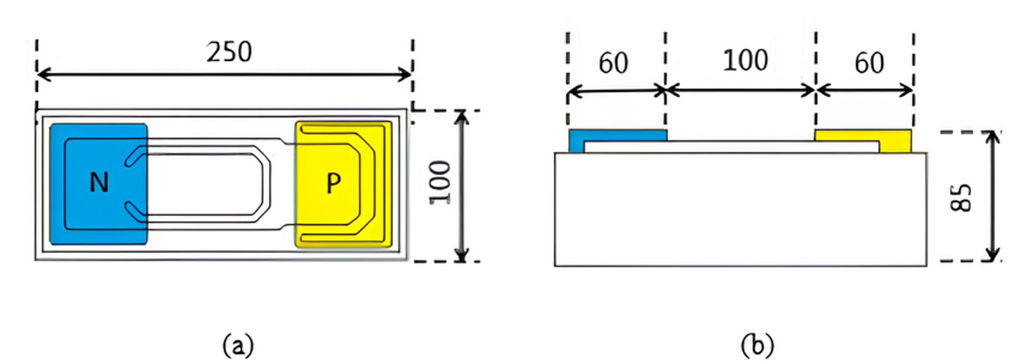
A two-layered electrode was used. The layer on top is silicone rubber (2401 mm2, 44 S/m [33]). The bottom layer consists of a saline gel (2500 mm2, 4 S/m [33]). It also includes a rectangular connector (108 mm2, 1000 S/m) affixed underneath the rubber pad (Fig. 1C).

Using the quasi-static approximation and the finite element technique (COMSOL Multiphysics Ver. 6.2) to solve Laplace’s equation [34], the electric potential produced by the current injected from a pair of electrodes (common bipolar tSCS) placed on the thorax was estimated using the following equation:

$$\beginc} \right) = 0,} \\ \end$$

(1)

where φ and σ denote the scalar potential and tissue conductivity, respectively. The electric field \(\overrightarrow\)=-∇φ was calculated in each element. There were 7,139,950 tetrahedral elements. The top 0.01% outliers were removed from the sorted E-field intensity produced by potential mesh errors [35]. The results were numerically stable relative to a finer mesh.

For bipolar tSCS, the electric field strength was obtained for a pair of electrodes. In the case of tISCS (Fig. 1D), the amplitude-modulated envelope (EAM) is generated from the vector sum of the two resultant electric fields (\(\overrightarrow_}\) and \(\overrightarrow_}\)), each corresponding to a pair of electrodes driven by an independent current source. The electric fields at location \(\overrightarrow\) are represented by \(\overrightarrow_}\) (\(\overrightarrow\)) and \(\overrightarrow_}\) (\(\overrightarrow\)). If |\(\overrightarrow_}\)| >|\(\overrightarrow_}\)| and the angle \(\alpha\) (angle between |\(\overrightarrow_}\)| and |\(\overrightarrow_}\)|) is lower than 90°, the modulation depth is expressed by [8, 17]

$$\begin \left| _} \left( } \right)} \right| \hfill \\ \quad = \left\c} _ \left( } \right)} \right|} & _ \left( } \right)} \right| < \left| _ \left( } \right)} \right|cos\alpha } \\ _ \left( } \right) \times \frac_ \left( } \right) - \vec_ \left( } \right)} \right)}}_ \left( } \right) - \vec_ \left( } \right)} \right|}}} \right|} & \\ \end } \right. \hfill \\ \end$$

(2)

The direction of one vector must be flipped if the angle is greater than 90°. The Eq. (3) provides an expression that uses the EF vector (\(_\left(\overrightarrow\right)\), \(_\left(\overrightarrow\right)\), \(_\left(\overrightarrow\right)\)) to obtain the maximum intermodulation depth intensity, corresponding to the direction of maximum modulation [36].

For the conventional tSCS, we used a bipolar montage with a midline orientation and inter-electrode distance of 2.5 cm [33, 37]. The electrode positions for tISCS were determined through a quasi-optimization process, described in the next subsection. The total injected current was fixed at 2.5 mA for conventional tSCS and tISCS [38]. As a result, the current per electrode pair in tISCS is halved relative to conventional tSCS. To ensure a fair comparison, we also implemented a two-pair in-phase bipolar tSCS configuration (referred to as 2-tSCS), matching both the number of electrodes and the current density used in tISCS. The electrode positions for 2-tSCS were set identically to those used for tISCS. It is important to note that the choice of maximum injected current does not affect the generalizability of the results, as the electric field magnitude in the model can be scaled linearly with the injection current intensity. Finally, we included an intuition-based montage for tISCS that was not derived from the optimization process but was instead adapted from conventional tSCS, using the same inter-electrode distance [33]. This montage serves as a baseline reference that might reasonably be chosen in practice without computational guidance.

The leadfield matrix \(}}_}}\) is a linear mapping from the injected current \(}}_}}\) to the resulting electric field \(\overrightarrow \left(p\right)\) at mesh node \(p\):

$$\overrightarrow \left(p\right)=}}_}}}}_}}.$$

(3)

To build the precomputed leadfield matrix \(}}_}}\), an electrode was fixed as the return in the center of the thorax, and a unit current was sequentially injected through each electrode distributed around the thorax for a total of 162 electrodes (6 vertical \(\times\) 27 horizontal positions). The simulations were carried out in COMSOL Multiphysics (v6.2) on an Intel(R) Xeon(R) W-2295 processor (3.00 GHz, 128 GB RAM), requiring roughly 30 h of computation. The resulting matrix, with dimensions corresponding to 162 montages × 3 field components × 7,139,750 mesh elements, enables rapid prediction of the electric field \(\overrightarrow \left(p\right)\) for any linear combination of input currents \(}}_}}\).

In the first step, we performed a brute-force search over a randomly sampled subset of montages candidates (quasi-optimization) to enable unbiased global exploration, ensuring that potentially effective electrode placements around the thorax were not overlooked. Specifically, 50,000 montages were sampled from a grid of 162 candidate electrode positions surrounding the thorax (Sect. 3.1). Two metrics guided the optimization: maximizing target intensity and maximizing focality [17, 39]. These objectives showed a trade-off that formed a Pareto front, consistent with prior findings (Fig. 2B). The Supplementary Material shows that quasi-optimization is stable for subspaces of more than 10,000 montages.

Optimisation procedure. A A total of 162 electrodes are used to build the leadfield matrix, B amplitude-modulated envelope (EAM) are obtained from a total of 50,000 random electrode combinations using the leadfield matrix. A Pareto front is formed from the trade-off between the maximum intensity of EAM in the spinal cord and the ratio of EAM between the spinal cord and skin (or muscle)

In the second step, we constructed a reduced subspace by retaining the most influential electrodes identified during global exploration (the “relevant electrode map,” Sect. 2.6), and then exhaustively evaluated all montage combinations of a 44-grid positions, as shown in Sect. 3.2.

From Eq. (3), the target intensity metric was

$$}_(\text)}=\text\left|}}_}\left(\text\right)\right|,$$

using only the z-component in the spinal cord because the target dorsal column fibers are assumed to align with the z-axis [40].

Focality was defined as the ratio of spinal-cord modulation to peak modulation in off-target tissues (skin and muscle):

$$}_(\text/\text)}=\text\left|}}_}\left(\text\right)\right|/\text\left|}}_}\left(\text\right)\right|,$$

$$}_(\text/\text)}=\text\left|}}_}\left(\text\right)\right|/\text\left|}}_}\left(\text\right)\right|.$$

The terms \(}_\left(\text\right)\) and \(}_\left(\text\right)\) represent the modulation depth along the direction of maximum modulation [36]. Because cutaneous nociceptors and muscle fibers are likely to align with this direction, these definitions yield a conservative estimate of focality.

We propose reducing the total number of potential electrode positions by introducing the “Relevant Electrode Map”, which shows the most influential positions. Figure 3A presents a 2D map displaying all electrode positions. Figure 3B shows the process used to identify the most relevant electrode positions. Each montage was assigned a score. A score of one point corresponds to montages on the Pareto front (green dot) derived from 50,000 random montages based on the 162-grid. A score of two points was assigned to the best-performing montage among them (red dot). These scores are accumulated over six repetitions and then normalized to generate the final Relevant Electrode Map.

Influential electrode positions in the grid. A Representation of electrode positions in a plane, B outline to obtain the Relevant Electrode Map