The workflow involving computational hemodynamic analysis, morphological analysis, and radiomic analysis is schematically summarized in Fig. 1.

A diagram showing the overall workflow of our data analysis

The institutional review boards at XXX and XXX approved our study protocol as a secondary analysis of existing data. Thus, informed consent was not required.

Thrombosed IAs were identified from an internal database at XXX. All imaging data were acquired using HR-MRI protocol, with a 3 T scanner (Magentom Skyra, SIEMENS) between May 2018 and December 2024. As part of the imaging protocol, T1-weighted (T1) and T1 + Gadolinium (T1 + Gd) sequences were obtained. T1 + Gd images were acquired 5 min after administering 0.1 mmol/Kg gadolinium-based contrast agent (Gadavist, Bayer Pharmaceuticals, Whippany, NJ; Supplementary Material). Images were isotropically resampled and spatially registered following a previously published protocol [14]. The analysis included patients with saccular and fusiform IAs with evidence of IST. Dissecting aneurysms may have been included in the analysis, as in some instances it is impossible to determine the exact location of the thrombus: intramural versus intrasaccular, despite the typical onion-skin appearance of the multilayered thrombus wall of dissecting aneurysms [2]. Demographic information was retrieved from electronic medical records.

To perform three-dimensional (3D) segmentation, an open-source processing software package (3D Slicer, version 5.6.1,https://www.slicer.org/) was used to mask the extent of each IA using T1 and T1 + Gd images [15]. Specifically, the segmentation process involved delineating the aneurysm and its parent vessels in T1 and T1 + Gd images. Digital subtraction angiography (DSA), magnetic resonance angiography (MRA) or computed tomography angiography (CTA) were used for quality control of the aneurysm boundaries.

Segmented masks in 3D Slicer were converted to a triangulated surface representing the IA vessel geometry. Then, a stereolithography (STL) file was generated for each IA model; each STL file was imported into a commercial software package (3-Matic V.16, Materialise Inc. Leuven, Belgium) for surface quality enhancement. Following a published method [16], an IA sac was first isolated from each triangulated vessel surface (i.e., the vessel model mentioned above). Then, aneurysm volume, aneurysm height, aneurysm width (i.e., maximum width along the direction that is perpendicular to the flow entering the aneurysm), aspect ratio (height/width), parent vessel diameter, and size ratio were calculated.

Other details of the morphological analysis are similar to those used in other publications (e.g [17,18,19]).,, and are provided in Supplementary Materials for completeness. Morphological metrics were computed using in-house Python scripts (Version 3.8) derived from Visualization ToolKit (VTK, Kitware, NY, USA).

CFD simulations were performed for each IA, following published protocols [20,21,22], as shown in Fig. 1. Similar CFD simulation protocols have been cross-verified against phase-contrast magnetic resonance angiography (PC-MRA) and ultrasound Doppler velocimetry for aneurysmal flow quantification [23,24,25,26,27].

Processed vessel geometries (see Model Creation Section above) were augmented with cylindrical flow extensions (minimum length: 10× vessel diameter) at all inlets/outlets using the Vascular Modelling Toolkit (VMTK v1.4, www.vmtk.org) to minimize boundary effects. Then, TetGen (Version 1.4.2) was used to generate unstructured 3D tetrahedral (volumetric) meshes for subsequent CFD simulations. All meshes contain five boundary layers with around 0.5–1.0 million elements. A mesh sensitivity analysis was conducted, and we concluded that appropriate mesh density was achieved.

The generated volumetric meshes were processed to solve transient Navier–Stokes equations using FLUENT (Version 21, Ansys Inc., PA, USA). Blood was modeled as an incompressible, laminar, Newtonian fluid with a dynamic viscosity of 0.004 Pa·s and a mass density of 1040 kg/m3. All arterial walls were assumed to be rigid, with a no-slip boundary condition.

Suited pulsatile flow (rate) waveforms were implemented as the inlet boundary condition, depending on the anatomical locations of selected aneurysms (e.g., from MR flow measurement in [28]). Zero-pressure boundary conditions were prescribed to all outlets. CFD simulations were performed for four cardiac cycles with 1000 (time) steps per cardiac cycle (0.001 s per time step). Twenty (20) sets of computed WSS and velocity data, temporally (equally) sampled from the last cardiac cycle, were used for the subsequent hemodynamic analysis.

Once CFD simulations were completed, the calculated WSS and flow fields became available for further analysis. At each point on the aneurysm surface, the WSS vector \(\:\tau\:=\left(_,_,_\right)\) was calculated by the Ansys Fluent. These vectors were averaged over 20 time points during the final cardiac cycle to obtain the time-averaged WSS (TAWSS), calculated as follows:

$$\:\frac\underset}\left|\tau\:\right|dt$$

(1)

where T is the duration of a simulated cardiac cycle and \(\:\left|\tau\:\right|\) stands for the magnitude of the WSS vector.

Using the generated TAWSS field, the endothelial cell activation potential (ECAP), which is linked to the potential of thrombus initiation [29] and the relative residence time (RRT) [30] can be computed for each point on the aneurysm sac:

Similarly, the oscillatory shear index (OSI) for each point on the aneurysm sac was calculated by determining the variation of the WSS vector over the cardiac cycle, as follows: [31]:

$$\:\frac\left(1-\frac}\tau\:\:dt}}\left|\tau\:\right|dt}\right)$$

(4)

In addition to WSS derived parameters, vortex analysis was performed to extract the vortex volume(VV) and number of vortex cores (NOC) to represent the gross aneurysmal hemodynamics.

As shown in Fig. 2, swirling flow eddies (i.e., recirculation zones) are present in the aneurysmal sac. Typically, flow eddies shift, break, and merge in space over a cardiac cycle. Using a published method [11, 32, 33], we first masked out the flow vortex core regions for each phase of the cardiac cycle (see the blue and red surfaces in Fig. 2A and B). Then, we calculated the degree of overlap (DVO) defined as the overlap ratio between the flow vortex core regions at two adjacent phases of the cardiac cycle (see Fig. 2C). Visualization of flow vortex cores over a cardiac cycle overlaid with time-resolved streamlines of the IA is shown in Figs. 2A-B.

An example showing complex flow disturbance in a saccular IA with a wide neck The degree of volume overlap (DVO) of flow vortex cores between two phases of a cardiac cycle: (A) the ith time-step (blue), (B) the (i + 1)th time-step (red), and (C) minimal flow vortex core overlaps indicating significant flow complexity. Velocity streamlines show the overall flow pattern at each phase

Sections 2 and 3 of Supplementary Materials include more WSS and flow vortex metrics details. These metrics were calculated using in-house Python scripts (Version 3.8) derived from the open-source VTK/VMTK (Version 1.4) software package.

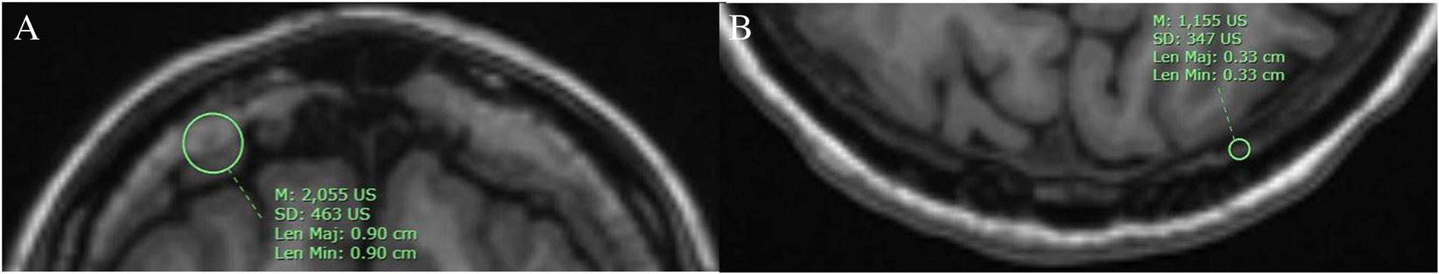
In 3D slicer, the thrombus boundaries were identified and isolated. A senior investigator (XXX) adjudicated the boundaries of the thrombus using DSA and MRA. HR-MRI was then used to isolate both the free aneurysm wall and the portion of the wall adjacent to the intrasaccular thrombus, as illustrated in Fig. 3.

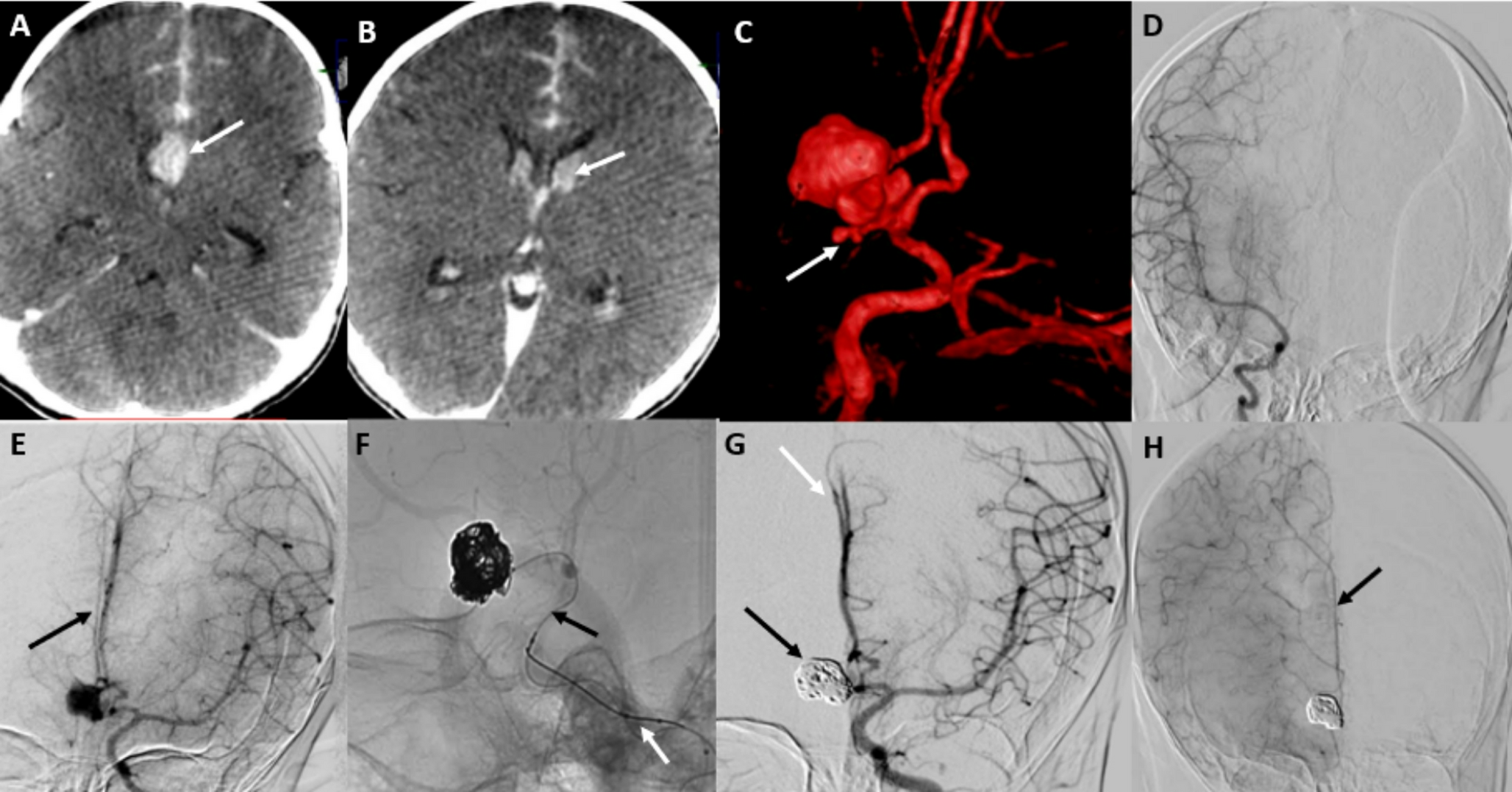
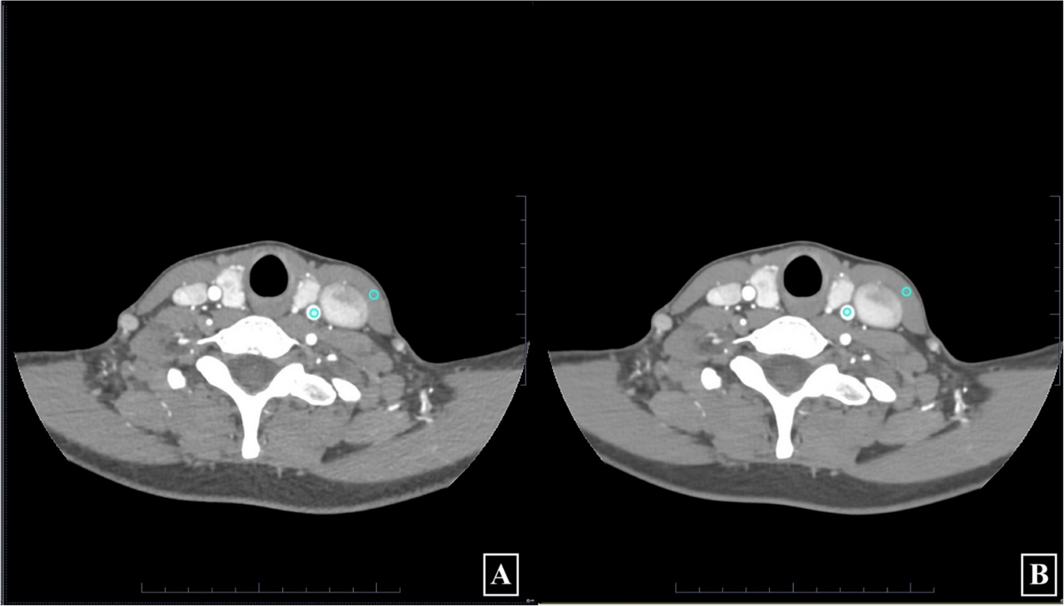
A terminal internal carotid artery (ICA) saccular aneurysm (A) with intrasaccular thrombosis (white star) is identified (arrowhead) in high-resolution magnetic resonance imaging (HR-MRI). Likewise, a (D) cavernous ICA fusiform aneurysm with IST (white star) is visualized in HR-MRI (arrowhead). (B & E) The boundaries of the thrombus (white arrows, yellow circle) are then identified on magnetic resonance imaging (MRA). (C, F) The wall next to the thrombus (yellow circle) and free of thrombus (red circle) is isolated, and radiomics are extracted

Py-Radiomics (https://pyradiomics.readthedocs.io/en/latest/) was used to retrieve RFs from the aneurysm wall and the IST (Fig. 3). One hundred thirty (130) RFs were extracted, involving 19/130 shape features, 36/130 first-order features, and 75/130 second-order features. In the end, two sets of RFs were obtained for each IA, namely, enhancement from the aneurysm wall free of IST and enhancement from the aneurysm wall next to IST.

In this study, spatial registration/correspondence between radiomics and CFD analyses was automatically achieved by using a shared (image) segmentation mask as a reference. Specificially, both the radiomic features and CFD simulations were derived from the same 3D aneurysm model, which was manually segmented from the original HR-MRI VWI images. The model was then divided into wall and lumen components for the respective analyses.

Spearman’s correlation values were calculated between RFs of the wall and IA parameters under the following three categories: (1) IA morphology, (2) WSS-related metrics, and (3) flow vortex core-related parameters. The correlation analysis (i.e., corr function) was conducted using the Statistics toolbox under MATLAB (Mathworks Inc., MA, USA). A subgroup analysis was conducted between RFs and hemodynamic parameters among saccular and fusiform thrombosed IAs. A strong correlation was defined as Rho > 0.7. A p-value less than 0.05 was considered statistically significant.