This prospective study was approved by the institutional review board (M2024079), and written informed consent was obtained from all subjects. Eligible adults with a clinically indicated cervical spine MRI between January and June 2024 were included prospectively. The exclusion criteria included: No CT examination records within 2 weeks (n = 125); previous surgery or metal implant (n = 109); no CT reconstruction image available (n = 23); the main assessment is other than cervical spondylosis, including spinal tumors (n = 15), myelopathy (n = 45), fractures (n = 6), atlantoaxial dislocation (n = 21), and cervical tuberculosis (n = 1). Finally, 137 patients with cervical spondylosis were continuously recruited for the study. The flowchart of patient inclusion and exclusion is shown in Fig. 1.

All MRI scans were performed using a 3.0-Tesla scanner (uMR 880, United Imaging Healthcare) with a 16-channel head and neck coil. The 3D-FRACTURE sequence has five in-phase echoes, isotropic voxels (voxel size 0.67 × 0.67 × 0.67 mm), and a field of view of 220 × 200 mm. MRI images with contrast like CT images were acquired by multiple echo sequences with constant echo-spacing. The five echo sequences acquired with the same resolution were set with different echo times (2.26, 4.49, 6.71, 8.93, and 11.15 ms). The echo train length was 33, the pixel bandwidth was 650 Hz/pixel, the acquisition matrix was 288, and the flip angle was 15°. A pre-saturation band was added to alleviate the movement artifacts caused by respiration and swallowing. This process was carried out by the MRI technologist based on their experience, adjusting the placement of the pre-saturation band to optimize artifact reduction while maintaining image quality. Details are provided in the Supplementary Material (Part 2). The overall scanning time of the FRACTURE sequence ranged between 3.50 and 4.25 min.

Custom MATLAB R2021b(R) was utilized for multiple echo data analysis to transform the CT-like images in two steps. First, a magnitude summation of all echo amplitudes was performed to improve the signal-to-noise ratio, leveraging the cumulative effect of the five echoes. Image contrast was enhanced as the signal decreased from the first to the fifth echo to maintain a high signal-to-noise ratio. Second, the grayscale of the cumulated images was inverted, resulting in a CT-like contrast of the bone cortex [8].

The cervical spine CT was performed using a 64-slice scanner (Somatom Definition Flash, Siemens) with open care dose 4D. The parameters were consistent with those of routine scans without adjustment: 120 kVp; tube current of 1000 mAs; slice thickness, 3.0 mm; pitch, 0.6; delay, 2 s; scan time, 4.32 s; rotation time, 0.5 s. Image data were reconstructed using a bone window (H60) and a soft tissue window (H40) with a layer thickness of 1 mm and a field of view of 200 × 200 mm. The CT scans acted as the reference standard for the presence of osteo-degenerative changes, which is widely recognized for its superior spatial resolution and excellent contrast in imaging bone structures [10].

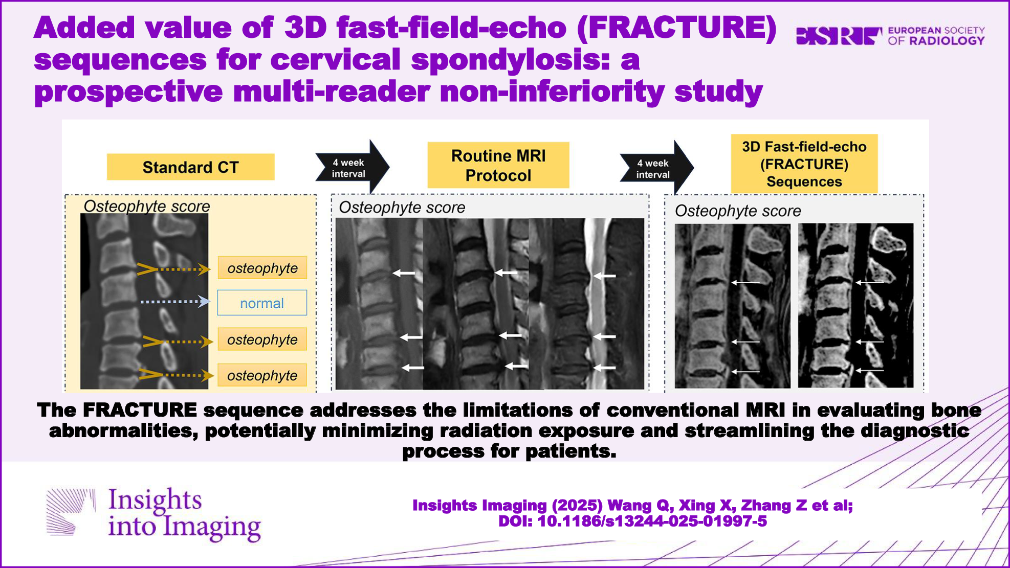
All data post-processing and collation work is done by an independent technician (Z.Z.). The datasets were anonymized and randomized for assessment. Three radiologists with different expertise levels (X.X., X.J., and Q.W. with 17, 9, and 5 years of experience, respectively) evaluated the same datasets independently. Before the multi-reader evaluation process, a 1-h seminar session was conducted by a specialist in musculoskeletal radiology (N.L.) with 20 years of experience using CT images of 15 patients outside the cohort. Considering that OPLL can be confused with white line artifacts along the posterior vertebral body edge, especially when window width and level settings are inappropriate, this is an important focus of this section, clarified through expert explanation. A detailed distinction with illustrations can be found in Part 3 of the Supplementary Material. The evaluation process consisted of three stages: CT, conventional MRI, and FRACTURE, with a 4-week interval between stages. After evaluating the CT scans, differences between the three readers were resolved by discussion, which further ensured consistent evaluation criteria among the three readers. The location of the abnormality and diagnostic confidence were recorded for each assessment in the MRI and FRACTURE stages.

The evaluation process and diagnostic criteria are shown in Fig. 2. Each case was evaluated using an anonymous questionnaire concerning osteophytes affecting the central spinal canal, bony foraminal stenosis, and OPLL. The observers could adjust the window width and level settings. Axial and sagittal images could be interactively referenced using position guidelines. The questionnaire focused on the cervical spondylosis bone structure assessed by CT while disregarding aspects clearly shown by routine MRI, such as disc herniation and spinal cord signals.

The evaluation process and diagnostic criteria diagram. Three major bone abnormalities of cervical spondylosis were evaluated: osteophytes, bony foraminal stenosis, and posterior longitudinal ligament ossification. The observers were allowed to make routine image adjustments during the evaluation. Two sets of FRACTURE sequences with different window widths and contrasts were presented

Detailed evaluation criteria were as follows: (1) Osteophytes involving the central vertebral canal were defined as those on the posterior lower or upper margin of the vertebral body. Equal vertebral signals were shown on conventional T1- and T2-weighted images. Each reader evaluated four intervertebral spaces (C3-4, C4-5, C5-6, and C6-7) and recorded the presence of osteophytes. (2) Bony foraminal stenosis was visually detected based on the shape of the foramina. Normal foramina are oval with smooth bone margins. Positive foramen stenosis was determined when visual changes in the foramen shape at the leading or trailing edge were noted. Advanced osteophytes might lead to occlusion. Stenosis due to disc herniation was not considered. The diagnosis was divided into eight sites (C3-4, C4-5, C5-6, and C6-7 on both sides). (3) OPLL appeared on CT images as a high-density posterior margin of the vertebral body or intervertebral space and was diagnosed at 11 locations (C2, C2-3, C3, C3-4, C4, C4-5, C5, C5-6, C6, C6-7, and C7). The ossified object could be in the center or to one side of the cross-sectional image and could appear as a typical layered structure or an isolated point-like ossification shadow in sagittal images. The OPLL MRI signal is identical to that of the bone cortex.

All diagnoses were compared to the reference to count the number of true positives. The bone abnormality score was calculated as the number of correct diagnoses at each site. That is, the number of true positive or true negative cases detected by the alternative at each assessment site, with CT results as the gold standard (CT is a perfect score). According to the number of sites mentioned above, the maximum scores for the three bone abnormalities (osteophytes, bony foraminal stenosis, and OPLL) were 4, 8, and 11. If the diagnosis was consistent with CT, the site was counted as one point, and zero if inconsistent. The higher the score of conventional MRI and FRACTURE sequence, the more equivalent to the diagnostic effect of CT, whereas the lower the score, the higher the proportion of false positive/false negative.

The diagnosis confidence was recorded using a 5-point Likert scale (a higher score means greater diagnostic confidence: 1 = least confident, 5 = strongest confidence). The overall diagnostic confidence for each patient was calculated by averaging the diagnostic confidence in all assessed sites with bone abnormalities.

Data was analyzed using MedCalc Statistical Software, Version 20.022 (MedCalc Software Ltd.). The numerical agreement among readers was assessed by the exact Fleiss Kappa, as it assigns greater penalties to larger discrepancies in ordinal ratings [13]. The square-weighted Cohen’s Kappa was used to assess the consistency between the MR protocol and the reference criteria. The reproducibility level was divided into excellent (> 0.9), good (0.7–0.9), moderate (0.5–0.7), and poor (< 0.5). A value of 0.7 was considered the lowest limit for good internal consistency of the test. To determine the distribution of bone abnormalities and diagnostic confidence scores, the Shapiro-Wilk test was performed, revealing non-normal data distribution and necessitating the use of non-parametric tests. The bone abnormality scores were compared using the Wilcoxon signed-rank matched-pairs test. The diagnostic confidence scores were analyzed using the Mann–Whitney U test. A significance level (α) of 0.05 was used. The McNemar test was selected to compare the diagnostic performance of routine MRI and FRACTURE sequences, as it is specifically designed for paired binary data. Non-inferiority analysis compared the image evaluation (osteophyte, bony foraminal stenosis, and OPLL scores), treated as continuous variables, to CT (reference standard). Since the score was derived from the number of correct diagnoses, the non-inferiority margin (−Δ) was set to 1, which is generally not expected to significantly impact clinical decision-making. We calculated that a sample of 98 would provide 80% power to detect non-inferiority at a one-sided alpha of 0.05, based on assumed effect size and variability from prior studies. To mitigate potential data loss and enhance the generalizability of our findings, we included additional cases.