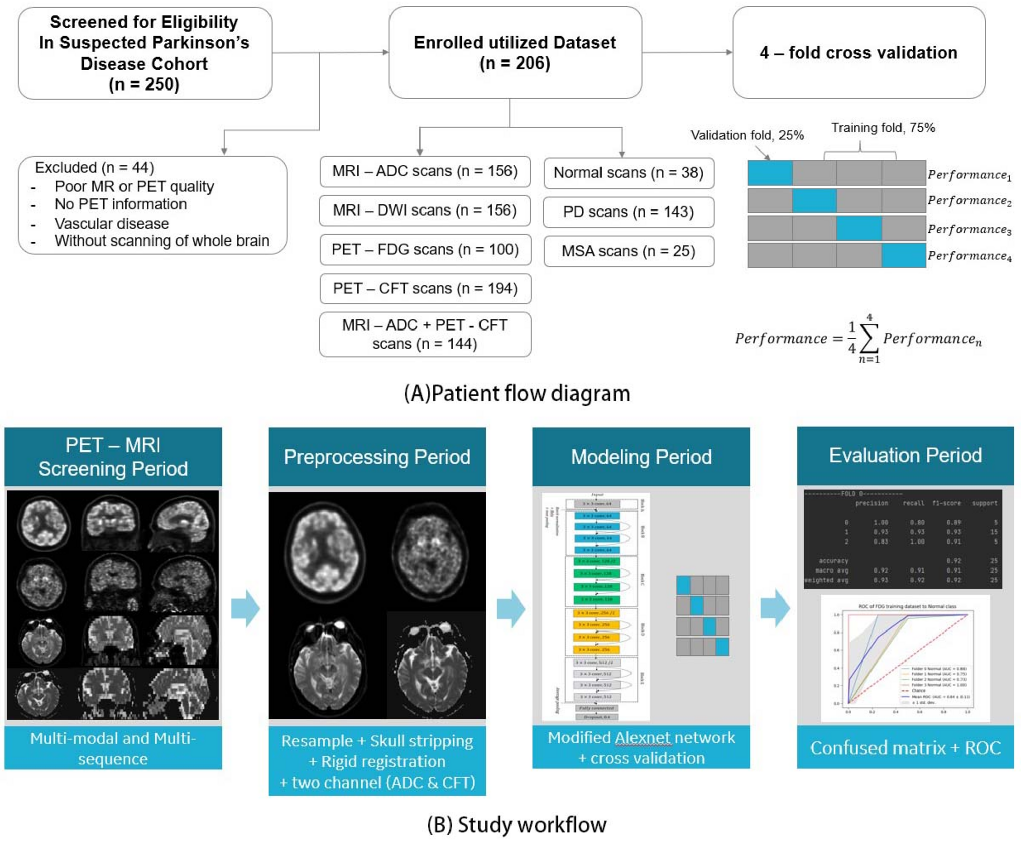
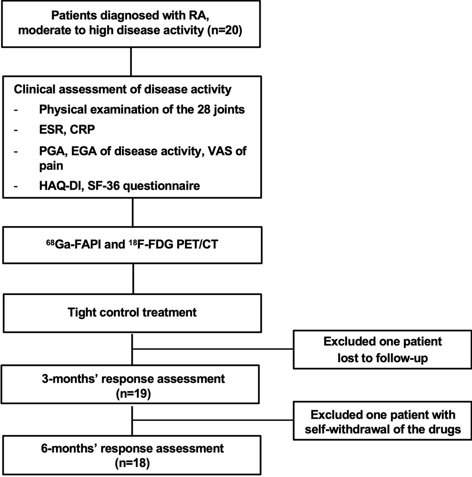
In this retrospective study, we enrolled patients who underwent positron emission tomography / magnetic resonance (PET/MR) imaging at the People’s Liberation Army General Hospital. Imaging was performed on a GE Healthcare PET/MR scanner (SIGNA™, GE Healthcare, Milwaukee WI, United States). The inclusion criteria were as follows: (1) fulfilling the diagnosis of PD and MSA according to the clinical criteria [17, 18]; (2) an interval between 11C-CFT and 18F-FDG PET/MR imaging of fewer than two weeks; (3) clinical follow-up at least six months after the initial PET/MR imaging without change in diagnosis. Exclusion criteria were (1) poor PET/MR image quality; (2) lack of recorded PET information; (3) evidence of vascular disease on computed tomography (CT) or MRI; (4) incomplete whole brain scanning. Of the two hundred fifty patients screened for eligibility, 44 were excluded due to poor image quality, insufficient PET information, signs of vascular disease, or incomplete brain coverage. Ultimately, 206 patients were included in the analysis, comprising 143 cases of PD and 25 cases of MSA. In addition, 38 volunteers without any identifiable neuropsychiatric diseases or symptoms were recruited to form the normal control (NC) group, as shown in Fig. 1A.

The workflow for this study

The workflow of this study is presented in Fig. 1 and consists of four major components: (i) image acquisition, (ii) image preprocessing, (iii) single-modal and multi-modal training and cross-validation, and (iv) evaluation, as illustrated in Fig. 1B.

The study cohort included 119 male and 87 female subjects, with an average age of 60 ± 14 years and an average weight of 67 ± 10 kg. This study was approved by the Chinese PLA General Hospital Human Ethics Committee, and all participants provided written informed consent prior to undergoing the PET/MR examination.

Prior to undergoing the 11C-CFT PET/MR scan, patients were required to abstain from medication for 12 h to prevent interference with dopamine transporter binding. Immediately after tracer administration, 20 milligrams of furosemide were injected. 50 minutes following the intravenous injection of 11C-CFT (180–370 MBq), three-dimensional (3D) MR and PET scans were acquired using an integrated whole-body PET/MR system. During this session, a multiparametric MRI examination of the brain was performed simultaneously within a 15 min single-bed PET scan, including both T1-weighted (T1w) and T2-weighted (T2w) sequences focused on the brain.

The 18F-FDG PET/MR scan was conducted on a different day, either before or after the 11C-CFT scan but within a two-week interval. Prior to the 18F-FDG acquisition, all participants fasted for at least 6 h and refrained from taking any medications that could affect brain metabolism for at least 12 h. An 18F-FDG dose of 0.1 mCi/kg (3.7 MBq/kg) was injected intravenously after confirming that the participant’s blood glucose level was ≤ 200 mg/dL. Participants then rested in a quiet, dimly lit room both before and after the injection until image acquisition commenced. The imaging parameters and data reconstruction settings for the 18F-FDG PET/MR scan were similar to those used in the 11C-CFT scan.

Image preprocessing was performed using Python (version 3.6) and SimpleITK (version 2.1.1) and involved several steps. Firstly, all 3D images were resampled via linear interpolation to achieve a uniform voxel spacing of \(\:1.0\times\:1.0\times\:1.0\:^\). Secondly, skull-stripping was applied to remove the skull, leaving only the soft brain tissue [19]. Thirdly, the Block Matching algorithm for global registration [20] was utilized to ensure the comparability among all CFT, FDG, ADC, and DWI images. This registration process transformed all images into a common space, aligning corresponding brain substructures at identical coordinates across participants. Consequently, the registered PET and MRI images could be directly concatenated as multimodal and multisequence data for model training or testing.

DL has been successfully applied in various medical fields, including lesion segmentation, CT image reconstruction, and lung cancer staging, et al.

ResNet, short for Residual Network, is a specific type of neural network that was introduced in [21]. Deep neural networks typically stack additional layers to solve complex problems, leading to improved accuracy and performance. For example, in image recognition, the first layer may learn to detect edges, the second to identify textures, and the third layer to recognize objects. However, it has been found that as the depth of the CNN increases, the performance of the CNN model tends to degrade [21]. The challenge of training very deep networks has been significantly mitigated with the introduction of ResNet, which is made up of Residual Blocks. The first key difference is that there is a direct connection that skips some layers (which may vary in different models) in between. This connection is called the “skip connection” and is the core of residual blocks. Due to this skip connection, the output of the layer is different now. The skip connections in ResNet solve the problem of vanishing gradient in deep neural networks by allowing this alternate shortcut path for the gradient to flow through. The other way that these connections help is by allowing the model to learn the identity function, which ensures that the higher layers will perform at least as well as the lower layers.

Due to the very limited number of training data, ResNet18 was utilized in this project, which can achieve good performance for three classifications. ResNet18 is a 72-layer architecture with 18 deep layers. At the end of model, dropout rate is set to 0.4 to improve robustness. The architecture of this network is aimed at enabling large amounts of convolutional layers to function efficiently. The introduction of residual blocks overcomes the problem of vanishing gradients through the implementation of skip connections and identity mapping. Identity mapping has no parameters and maps the input to the output, thereby allowing the compression of the network at first and then exploring multiple features of the input. Figure 2 shows the layered architecture of the ResNet18 CNN model.

An illustration of the architecture of ResNet18

For inputs to the two-dimensional (2D) neural network classifier, we extracted 2D image slices from 3D PET and MRI scans. A 3D image can be viewed from three perspectives—axial, coronal, and sagittal—corresponding to the three standard anatomical axes. We identified key positions within a 3D image where the corresponding 2D slice most clearly revealed morphological differences in brain atrophy between PD cases, MSA cases, and normal controls. These key positions were individually selected for each image: the center of the X-axis for the axial view, the center of the Y-axis for the coronal view, and the center of the Z-axis for the sagittal view (see Fig. 3).

2D Images at Key Positions for Three Views from a preprocessed PET CFT scan. 1st column: axial view; 2nd column: sagittal view; 3rd column: coronal view

During training, slice indices was randomly extracted within a range of 10 slices around these key positions in each of the three views (Fig. 3). For validation and testing, 2D slices were constructed precisely at the key positions for each view. For every testing case, the three 2D slices (one from each view) were sequentially fed into the trained network, and the final predicted label was determined by a majority vote among the three slices. If at least two out of three 2D slices indicated a PD label, the entire 3D scan was classified as “having PD.”

For the multi-modal and multi-sequence modeling dataset, 6 slices of images are composed of 3 slices from a preprocessed MR-ADC scan and 3 slices from the same patient’s preprocessed PET-CFT scan. Since a rigid registration was performed during the preprocessing phase, these 20 slices of images could be directly concatenated into a synthesized dataset.

One of the main sources of variability in DL originates from the difference between the observed samples of the dataset and the real distribution of the dataset. The fact that the learning step of the algorithm is performed on only a part of the distribution can affect the reproducibility and, particularly, the replication of the results. To avoid bias in the data selection, strategies called “Cross-Validation” are performed. These strategies consist in dividing the dataset into several folds, then assigning these folds to the training, validation, and testing sets. The cross-validation strategies permit one to address variability in the data. In this study, we chose 4-fold cross-validation. Data are randomly partitioned into four folds of roughly equal sizes, and in each round of the cross-validation process, 3 of the folds are used for training the model, and the rest fold is used for testing. The whole process is repeated four times such that all folds are used in the testing phase, and the average performance on the testing folds is computed as an unbiased estimate of the overall performance of the model, as shown in Fig. 1.

We trained the network on the framework of Pytorch 1.10.1 version. The graphic card used for training was NVIDIA Quadro P3200, which has 5 GB memory. In addition, the optimizer we used is the Adam optimizer, and the learning rate is set to be \(\:^\). We set the batch size as 16 and ran 50 epochs on the training set. For the four single-modal datasets, the whole training process took nearly 2 h. For the one multi-modal dataset, the whole training took around 2.5 h.

The PET/MR dataset in this study contains three classes, and we treated this multi-label classification problem as multiple binary classifications. In this setting, the classification performance is evaluated in each class. Each of the metrics is computed for every divided class. Specifically, for the \(\:j\) class \(\:_\), \(\:_,__\) denote the number of true positive, false positive, true negative, and false negative test samples concerning \(\:_\). We reported four metrics, i.e., \(\:Precision,\:Recall,\:F1\) score and AUC for each disease:

$$\:_=\frac_\times\:recall}_}_+recall}_}$$

(3)

Also, for an overall comparison of all classes, we report the macro average of the metrics. The macro average of binary classification metric: \(\:B\in\:Precision,\:Recall,\:F1\) can be defined as:

$$}}}(h) = \sum\limits_^q B \left( ,F,F} \right)$$

(4)

Where \(\:q\) denotes the number of samples.

The area under the ROC curve (AUC) value was calculated to evaluate the classification performance.

All analyses were performed using SPSS (version 22.0; IBM, Armonk, NY). Quantitative variables are presented as averages and ranges, while categorical findings are expressed as numbers and percentages. For quantitative data with a normal distribution, subgroup differences were compared using a t-test; for non-normally distributed data, the Mann-Whitney U test was employed. Differences between categorical variables were evaluated using chi-squared tests. Statistical significance was defined at the 5% level (P < 0.05).