Electrophysiology and behavioral monitoring

All animal procedures were approved by the University of Pittsburgh Institutional Animal Care and Use Committee in accordance with the guidelines of the US Department of Agriculture, the International Association for the Assessment and Accreditation of Laboratory Animal Care and the National Institutes of Health. Data collection was performed using LabVIEW (2014) and MATLAB (2024a). Three animals were trained on a center-out reaching task. We then implanted arrays in the motor cortex contralateral to the trained reaching arm. We recorded neural activity from the proximal arm region of the primary motor cortex (M1) in two male rhesus macaques (monkey E, aged 12 years; monkey D, aged 12 years) using a 96-electrode (1.0 mm electrode length) microelectrode array (Blackrock Microsystems). In a third monkey (monkey Q; male, aged 6 years), we implanted a 64-electrode (1.0 mm electrode length) array in the dorsal premotor cortex and a 64-electrode (1.5 mm electrode length) array in M1. The recorded neural signals were amplified and digitally processed using the TDT RZ2 system (Tucker–Davis Technologies). The digitized signals were bandpass filtered between 300 Hz and 3 kHz. We recorded neural activity as threshold crossings, where a threshold crossing was detected when the depolarizing phase of the voltage signal crossed a threshold of three times the root-mean-square (RMS) voltage. We estimated the RMS voltage of the signal on each electrode before each experiment while the monkeys sat calmly in a darkened room. We recorded 94.0 ± 1.1, 79.9 ± 1.6 and 96.7 ± 0.5 neural units (mean ± s.d.) from monkeys E, D and Q, respectively. This study was conducted between 8 and 18 months after array implantation for monkey E, 9 and 18 months after implantation for monkey D and 3 and 6 months after implantation for monkey Q.

During experiments, animals sat head-fixed (monkeys E and D) or head-free (monkey Q) in a primate chair in front of a visual display with both arms loosely restrained in a pronated posture. To reduce hand movements during the BCI trials and to ensure a consistent hand position, the monkeys placed their hand (contralateral to the array) on a horizontal ‘touch bar’. The touch bar was instrumented with either a contact sensor (Spectra Symbol; some sessions with monkey E) or a force transducer (monkeys E, D and Q; Mini40, ATI Industrial Automation, NC) to measure hand contact with the touch bar. Animals were required to maintain this contact throughout the trial. Releasing the bar or exerting force outside of a predetermined window resulted in an immediate failure of the trial. The target force window was calibrated relative to the weight of the animal’s hand resting on the force bar independent of any task condition. The size of the force window depended on the orientation of the touch bar with respect to the 6-degree-of-freedom torque cell. Monkeys E and D maintained a force within an 11.8 N window, and monkey Q maintained a force within a 1.3 N window. For all monkeys, we could measure very small changes in force. The position of the hand was tracked using an LED marker (Phasespace). Consistent with previous BCI experiments31, there was minimal arm movement or force production during BCI trials (representative session shown in Extended Data Fig. 8).

Behavioral tasks

For all behavioral tasks, trials were initiated by holding the touch bar for 250 ms. Upon initiation, a BCI cursor and a target were displayed simultaneously on the monitor. The cursor remained fixed at the center of the workspace for 500 ms (referred to as the ‘freeze period’), after which the cursor was placed under neural control. For all tasks, the animals were trained to move the cursor to acquire the presented target. The target was acquired when the cursor contacted the target (that is, no hold time was required). Animals received a liquid reward upon successful completion of a trial. Each animal performed the following BCI tasks, described in detail below—center-out task, two-target task, grid task, IT task and instructed path task.

Center-out task

Animals were required to move the BCI cursor from the center of the workspace to one of eight possible peripheral targets 90 mm from the center, arranged around a circle at 45° intervals. Animals were given 4 s to acquire the peripheral target. Failure to acquire the target within this time or failing the touch bar conditions (that is, releasing the bar or exerting force) resulted in a 2 s (monkeys D and Q) or a 5.5 s (monkey E) timeout. Targets were presented in a pseudorandom order such that each of the eight targets was presented and attempted once before any target was repeated. We used a block of 160 trials of the center-out task to calibrate the MoveInt decoder (see below).

Two-target task

Animals moved the BCI cursor to sequentially acquire two diametrically opposed peripheral targets (A and B). There were the following four possible target pairs: 0° and 180°, 90° and 270°, 45° and 225°, 135° and 315°. One target pair was tested in each session and was selected before the start of the session. These peripheral targets were placed 90 mm from the center of the workspace. There were nine experiments in which monkey Q was unable to acquire the peripheral targets at 90 mm, so we reduced the target distance to the greatest distance that the animal could acquire (80–85 mm). This task consisted of two steps. In the first step, the cursor and a peripheral target (pseudorandomly chosen to be target A or target B) simultaneously appeared on the screen, and the monkey had 4 s to acquire the target (Extended Data Fig. 9a, left). We refer to the target acquired in step 1 as the ‘start target’. In the second step, the diametrically opposed target appeared, and the monkey had 4 s to move the cursor from the start target to it, that is, from target A to target B or from target B to target A (Extended Data Fig. 9a, right). The trial was a success if the target in step 2 was acquired. Failing to acquire the second target led to a 5.5 s penalty, and all other failure modes resulted in a 2 s (monkeys D and Q) or a 3 s (monkey E) penalty.

Grid task

This variant of the two-target task included additional targets for the second step. Starting with the same peripheral target pair as was used for the two-target task in that session, the animal first acquired one of the two start targets, selected pseudorandomly. For the second step, there were three possible target locations—the diametrically opposed target or two targets orthogonal to the target pair axis (Extended Data Fig. 9b). The probabilities of the targets were weighted so that there were 100 total trials to the diametrically opposite target and 20 total trials to each of the other two targets. For each step, the animal had 4 s to acquire the target. Following the successful completion of the second step, the animal received a liquid reward. Penalty durations were as described for the two-target task.

IT task

This task was a variant of the two-target task in which the second step was to an IT, placed along an axis orthogonal to the target pair axis (Fig. 6). The location of the IT was selected for each experiment so that the animal could acquire it from both target A and target B (Extended Data Fig. 9c). To determine the excursion of the IT, we gradually increased the target distance from the center of the workspace in 10% increments of the peripheral target distance until the success rate began to decline. The final IT position was chosen to ensure both of the following: (1) the target location was aligned with the path of the flow field (Extended Data Fig. 9c, blue arrow) and (2) the success rate was high from both start targets. Across experiments, this procedure resulted in an IT position that was 31.2 ± 11.4 mm from the center of the workspace. The animals performed ~100 total trials (100.1 ± 0.3) of the IT task, moving from either start target to the IT (that is, A to IT and B to IT). These trials were used to estimate trajectory flexibility (‘Initial angle metric’).

Instructed path task

We modified the IT task so that the objective was to move the cursor along a path specified by a visual boundary around the start target and the IT (Fig. 7a). To succeed at the task, the animals were required to keep the cursor within the boundary as they acquired the IT. The boundaries were straight, capped cylinders that encased the allowable paths between the start target and the IT. The boundary edges were equidistant (ranging from 30 to 150 mm) from the target axis (that is, the line that connects the targets).

A trial of the instructed path task began with the presentation of the start target. After its successful acquisition, the IT and the visual boundary appeared simultaneously. Animals then had 4 s to acquire the IT (that is, the ‘acquire time’) without the BCI cursor touching the boundary to receive a reward. Failing the boundary requirement resulted in a time penalty that was 2 s plus the remaining acquire time. This trial structure ensured that animals would receive shorter time penalties for trials in which they were actively attempting to acquire the target and longer penalties for failing quickly.

The instructed path task started with a boundary size that required minimal modification of cursor trajectories for success. The first boundary was chosen to have a width of 110 or 120 mm, except for one session for monkey D (150 mm width) and two sessions for monkey E (80 mm width). Then, we gradually reduced the size of the boundary to encourage the animals to modify their cursor trajectories. The reduction happened in one of two ways. For all sessions with monkeys E and D, and 6 of 13 sessions with monkey Q, we evaluated the animal’s task performance every 25 trials and reduced the boundary’s width by 10 mm if the animal exceeded a 75% success rate. For the other 7 of 13 sessions of monkey Q, we evaluated the animal’s task performance every 25 trials and reduced the boundary size such that the new smaller size would yield a predicted 75% success rate. With both approaches, if the success rate failed to meet the 75% success rate threshold, we began evaluating performance in 50-trial blocks (including the 25 trials that were just evaluated). If the success rate threshold was not met in a given block, the boundary size would stay the same for another 50-trial block. The boundary was not increased once reduced, except in rare instances where the initial boundary width was too difficult for the animal. The animals performed an average of 501 ± 108 instructed path trials (Extended Data Fig. 6). For the final 100 trials, we kept the task parameters constant even if the animal met the success rate threshold. Experimental sessions that included the instructed path task are summarized in Supplementary Table 1.

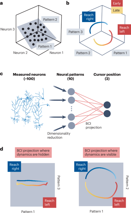
BCI mappings

To study temporal constraints on neural population activity, we sought to give animals moment-by-moment feedback on their neural trajectories. To accomplish this, the recorded neural activity was transformed into the position of a computer cursor. We used GPFA33 to transform the ~90D neural activity at each time step into a p-dimensional latent state. For all experiments, we used p = 10, as this has been found to capture most of the shared variability in the motor cortex during BCI control31.

Ideally, we would provide the animal visual feedback of all ten dimensions, but providing ten dimensions of feedback is challenging to configure experimentally. Instead, we provided visual feedback as a selected 2D projection of the 10D latent state. The 10D latent states were mapped to 2D cursor positions via BCI mapping. We used two types of BCI mappings defined below—MoveInt and SepMax. Unlike our previous BCI studies31,32, which mapped neural activity to cursor velocity, here neural activity is mapped to cursor position to establish a direct correspondence between the neural activity patterns and workspace location.

Extracting neural trajectories

To calculate neural spike counts, we binned threshold crossing events for each electrode channel in nonoverlapping 45 ms time windows. We used GPFA to extract the latent state at a given point in time \(}}}_\in ^\) from the spike counts \(}}}_\in ^\) at the recent past and current time points, where \(q\) is the number of neural units. GPFA defines a linear Gaussian relationship between latent states and spike counts as

$$}}}_|}}}_ \sim N(C}}}_+}},\,R),$$

(1)

where \(C\in ^\) specifies the relationship between the latent states and spike counts, \(}}\in ^\) is the mean activity of each neural unit and \(R\in ^\) is a diagonal matrix specifying the independent variances of the neural units.

Latent states are related across time using Gaussian processes. The neural trajectory for the ith latent state at time steps 1 to \(T\), \(}}}_=\left[_,\,\ldots ,_\right]\), is defined as

$$}}}_ \sim N(},_),$$

(2)

where \(_\in ^\) is a covariance matrix defining the relationship between the ith latent state at different points in time and \(i=1,\,\ldots ,\,10\).

The GPFA parameters \(C\), b, \(R\) and latent timescales in \(_\) were fit using the expectation-maximization algorithm, as described in ref. 33. For monkey E, a GPFA model was fit to the center-out trials to define the MoveInt mapping, and a separate GPFA model was fit to the two-target task trials to define the SepMax mapping (‘MoveInt mapping’ and ‘SepMax mapping’). For monkeys D and Q, a single GPFA model fit to the center-out trials was used to define the MoveInt and SepMax mappings. We included neural activity from target onset to target acquisition on successful trials and neural activity from target onset to the moment of failure on failed trials.

To extract the neural trajectories, first, we extracted the unsmoothed latent state,

$$}}}}_=^^(}}}_-}}),$$

(3)

where \(}}}}_\in ^\). The standard form of GPFA uses both past, current and future neural activity to estimate the current neural state33. Because we are presenting neural trajectories in real-time to the animals, we are limited to using past and current neural activity. We, therefore, designed a causal implementation of GPFA55 in which the latent state at the \(\)th time step is only determined by neural activity from the previous seven time steps (that is, \(t-6\) to \(t\), approximately 315 ms into the past), rather than neural activity from all past and future times. We concatenated the unsmoothed latent states for the previous seven time steps

$$}}}}_=}}}}_^,\ldots ,}}}}_^\right]}^,$$

(4)

where \(}}}}_\in ^\). Finally, the neural trajectories were extracted in real time as

where \(}}}}_\in ^\) is the estimate of the latent state at time \(t\) and \(M\in ^\) is a ‘smoothing matrix’ describing the contribution of past and current spiking activity on the latent state at time \(t\) (Extended Data Fig. 10). The contributions corresponding to time steps \(t-7\) and beyond were negligible relative to the contributions from more recent time steps (Extended Data Fig. 10). The smoothing matrix \(M\) is obtained from the model parameters \(C\), \(R\) and \(_\) (\(i=1,\,\ldots ,\,10\)) as described in ref. 33. The spike count history used to extract neural trajectories was reset to zero at the beginning of each trial. There were no ‘edge effects’ of estimating \(}}}}_\) related to this reset, as the touch bar hold time (250 ms) and the cursor freeze period (500 ms) occurring at the beginning of each trial were longer than the 315 ms spiking history used for the causal GPFA mapping.

Using the \(}}}}_\) extracted by GPFA, we specified a BCI mapping of the form

to convert \(}}}}_\) into a cursor position \(}}}}_\in ^\), where \(W\in ^\) is a weight matrix and \(}}\in ^\) is a positional offset. Each BCI mapping (MoveInt and SepMax) used a different W and c, defined below.

MoveInt mapping

Each experiment began with calibrating the MoveInt mapping. We used a gradual training process31 to determine the parameters to use for this mapping. This process consisted of a series of five blocks of 32 center-out trials, in which we updated the mapping parameters after each block, using all accumulated data up to that point. The first block consisted of passive observation trials, during which the cursor was moved to the peripheral targets under computer control. The cursor was moved at constant velocity (0.15 m s−1) straight to the target. The targets were presented in a pseudorandom order (~4 trials per target). Following the observation block, animals were given control of the computer cursor, but we attenuated the perpendicular error to discourage online movement corrections. The amount of perpendicular error attenuation was reduced in each block so that the animal had full online control of the cursor by the final training block. After the final block, we used the data from all five blocks to calibrate the MoveInt mapping.

The MoveInt BCI mapping was designed to provide animals with proficient cursor control such that they were able to move the cursor quickly and accurately to targets placed throughout the workspace. To identify the MoveInt mapping, we used linear regression (equation (6)) to solve for the parameters \(_}}\in ^\) and \(}}}_}}\in ^\) that best predicted the assumed intent of the animals given their neural trajectories. More specifically, mapping parameters were defined as

$$}}}_}=-_}\left(\frac\mathop\nolimits_^}}}}_\right),$$

(8)

where \(Z=[}}}}_,\,\ldots ,}}}}_]\in ^\) comprises the latent states estimated by GPFA, \(X=\left[}}}_,\ldots ,}}}_\right]\in ^\) comprises the associated intended cursor positions (see below) and \(n\) is the total number of time steps during the calibration trials.

The calibration data for each trial consisted of sets of }}}_\), xt} for two time epochs—the first epoch comprised three time bins of activity within each trial that captured baseline activity (\(_}}\)), and the second epoch comprised five time bins of activity within each trial that captured activity when the animal was engaged in the task (\(_}}\)). The details of which time bins comprised each epoch varied for each monkey and are described below. For all animals, n = ncalibration trials × (Tbase + Tengaged), where ncalibration trials is the number of calibration trials. Therefore, after each 32-trial block, n increased by 256 (that is, 32 × (3 + 5)) time steps.

For monkey E, the first time epoch consisted of the first three time bins (~135 ms) of the touch bar hold period. During this period, we assumed that the animal was not attempting to move the cursor and set xt = [0 mm, 0 mm]T. The second time epoch was five time bins in duration (~225 ms) immediately preceding the acquisition of the BCI target. During these time bins, we assumed that the animal intended that the cursor be placed at the target location (for example, xt = [90 mm, 0 mm]T for the rightward target). We found that these assumptions generally worked well for monkey E, whose neural activity was highly stereotyped during calibration.

For monkey D, using the above calibration approach led to MoveInt mappings that did not provide good cursor control (that is, the animal was not able to consistently acquire all targets). This is likely due to neural responses in the five time bins preceding the acquisition of the target that were more variable on a trial-to-trial basis than we observed for the other monkeys. Instead, we identified target intent for monkey D during the final five time bins of the freeze period because neural activity showed more target intent at that point in the trial.

Monkey Q tended to release and regrasp the force bar between trials, which led to some inconsistencies at the beginning of the trial until he settled into a stable grip for the remainder of the trial. To account for this behavioral variability at the beginning of the trial, we defined the first epoch as the first three time bins of the freeze period. The second epoch was defined in the same way as for monkey E.

SepMax mapping

The SepMax BCI mapping was designed to highlight projections of neural activity in which neural trajectories took markedly different paths through the latent space when moving between target pairs in the two-target task. We identified projections that jointly satisfied the following three objectives (Extended Data Fig. 10): (1) maximization of the separation between the midpoints of the A-to-B trajectories (\(}}}}_}}\)) and the B-to-A trajectories (\(}}}}_}}\)), (2) minimization of the trial-to-trial variance at the midpoints (\(_}}\) and \(_}}\)) and (3) maximization of the distance between the starting points of the A-to-B trajectory (\(}}}}_}}\)) and the B-to-A trajectory (\(}}}}_}}\)).

We first computed the trial-averaged starting points \(}}}}_}}\) and \(}}}}_\in ^\) for the A-to-B and B-to-A trajectories, respectively (Extended Data Fig. 10d). We then defined an axis connecting \(}}}}_}}\) and \(}}}}_}}\), along with its midpoint

$$}}=\frac}}}}_+}}}}_},$$

(9)

where \(}}\in ^\). For a given single-trial neural trajectory, we projected each of its latent states \(}}}}_\) (equation (5)) onto this axis. We defined the midpoint of the neural trajectory as \(}}}}__}\), where \(_\) is the time point at which the projection of \(}}}}_\) onto the axis was closest to m. The trial averages of \(}}}}__}\) for the A-to-B trajectories and the B-to-A trajectories are \(}}}}_}\in ^\) and \(}}}}_}\in ^\), respectively (Extended Data Fig. 10e). The covariance across trials of \(}}}__}\) for the A-to-B trajectories and the B-to-A trajectories are \(_}}\in ^\) and \(_}}\in ^\), respectively.

To identify the SepMax projection, we used an optimization procedure56 to identify a set of basis vectors to project the 10D neural trajectories into 2D cursor positions to satisfy the objectives mentioned above. Specifically, we sought to find an orthonormal set of vectors \(_}}=\left[}}}_,}}}_\right]\in ^\), which minimized the objective function:

$$J=-_}}}}_^(}}}}_}-}}}}_})+_}}}}_^\left(_}+_}\right)}}}_-_}}}}_^(}}}}_}-}}}}_}),$$

(10)

where \(_}},\,_}\) and \(_}}\) are scalar weighting factors. The first term of the objective function maximizes the midpoint separation, the second term minimizes the trial-to-trial variance and the third term maximizes the starting point separation. Thus, p1 is the dimension along which the A-to-B and B-to-A trajectories are separated, and p2 is the dimension along which the targets are separated (that is, the target axis).

Weighting factors \(_}}\), \(_}\) and \(_}}\) were used to specify the relative influence of the midpoint, covariance and starting point terms on the overall objective function value. For monkey E, each of these terms was set to 1. For monkeys D and Q, the weighting factors were chosen such that the identified projections were not dominated by any single objective. To find the weighting factors, each term in the objective function (ignoring \(_}}\), \(_}\) and \(_}}\)) was calculated for 10,000 different random orthonormal projections \(_}}\). We set each weighting factor to be the inverse of the range (that is, maximum value–minimum value) of that term. Objective function minimization proceeded as outlined in ref. 56, with a convergence criteria of \(\Delta J=^\), a maximum of 1,000 gradient iterations and a line search step size of 0.1. The SepMax mapping was calculated from the 160 trials of the two-target task or from the ~100 trials of the grid task to the diametrically opposed targets.

To make BCI control with the SepMax projection as intuitive as possible for the animal, we made the visual feedback as consistent as possible between the different BCI mappings. To determine the SepMax mapping parameters (\(_}}\) and cSM), we aligned the space defined by \(_}}\) with the animals’ workspace such that the starting points of the A-to-B and B-to-A trajectories in the SepMax mapping were at the same position as targets A and B in the cursor workspace. Specifically, we defined

where \(_}}\in ^\), \(A\in ^\), \(}}}_}}\in ^\) and m is defined in equation (9). The matrix

specifies a linear transformation involving three operations to provide intuitive visual feedback with the SepMax mapping. First, we scale the axes of \(_}}\). The scaling matrix \(S=\in ^\) is a diagonal matrix that scales the axes of \(_}}\), such that the distance between \(}}}}_}}\) and \(}}}}_}}\) is equal to the distance between targets A and B in the MoveInt mapping. Then, we optionally flip the projection about the target axis using the matrix \(O\in ^\) (Extended Data Fig. 10g,h). We want to orient the SepMax projection such that attempted movements move the cursor in the expected direction (for example, when the monkey intends to move up, the cursor moves up rather than down). To determine the sign of p1 that achieves this goal, we visually inspected the neural trajectories during the grid task (Extended Data Fig. 9b) in both orientations. We chose the sign of p1 such that the endpoints of the neural trajectories in the SepMax projection were closest to the associated target location (Extended Data Fig. 10g,h). This choice was made with the intent of reducing the cognitive burden imposed on animals when using the SepMax mapping. Finally, we rotated p2 so that it aligned with the workspace targets A and B. The matrix \(_\in ^\) rotates the projection through angle \(\theta\), where \(\theta\) is the angular difference between the axis connecting the workspace targets in the MoveInt mapping and the p2 axis.

Experimental flow

The experimental flow for a single session was the same for all monkeys. Each experiment began by calibrating a MoveInt mapping that captured the animal’s movement intention during the center-out task. The MoveInt mapping was then used during the two-target task or the grid task to identify the SepMax mapping for one target pair (Fig. 3). Then, we tested the flexibility of the temporal structure evident in the SepMax mapping with three experimental manipulations. First, we gave the animal visual feedback of the dimensions where temporal structure was evident by having the animal perform the two-target task using the SepMax mapping (Fig. 4). Then, we used the IT task to ask if the animal could produce time-reversed neural trajectories (Fig. 6). Finally, in the instructed path task, we directly challenged the animal to follow a prescribed path (Fig. 7).

The details of how we identified the SepMax projection varied somewhat for each monkey. For the majority of sessions for monkeys E and D, only a single target pair was tested. We selected the target pair to be tested pseudorandomly before the start of the experiment. We identified the SepMax projection for that target pair using either 160 trials of the two-target task or 140 trials of the grid task with the MoveInt mapping. If we used the grid task, only the ~100 trials to the selected target pair were used to identify the SepMax projection. For monkey Q, we used a different procedure because this monkey showed high variability in the separation of neural trajectories across sessions. We selected the target pair to be tested each day from 160 two-target trials comprising all four target pairs (that is, 40 trials per target pair) using the MoveInt mapping. The selection criterion balanced the desire to test each target pair across multiple sessions while also prioritizing target pairs with strong trajectory separation. After selecting the target pair to be tested, we identified the SepMax projection using the ~100 trials of the grid task to the selected target pair.

Once we identified the SepMax projection, the animals exclusively used the SepMax mapping to control the cursor for the remainder of the tasks in the session. To assess the persistence of temporal structure when it was provided as visual feedback to the monkey, the animal performed 100 trials of the two-target task using the SepMax mapping (Fig. 4). Next, we ran 50–100 trials of the IT task for each start target using the selected target pair while we adjusted the position of the IT. We used these trials to establish the location of the IT. After setting the position of the IT, we ran an additional 100 trials (100.14 ± 0.35 trials) of the IT task with both start target positions. These trials were used to estimate trajectory flexibility (Fig. 6; ‘Initial angle metric’). For the final task of each session, the animal performed ~500 trials (501 ± 108 trials) of the instructed path task. We reduced the visual boundary according to the animal’s success rate, as described above (Fig. 7; ‘Instructed path task’).

Analyses

We performed 135 experiments. We excluded a session if any trials were corrupted or lost during the data-saving process or if animal motivation issues prevented us from obtaining a MoveInt mapping that provided satisfactory control. Overall, this exclusion process resulted in excluding two sessions due to lost or corrupted data and four sessions due to low motivation. We analyzed 111 two-target sessions with the SepMax mapping (50, 40 and 21 sessions for monkeys E, D and Q, respectively). A subset of those sessions also included the IT and the instructed path tasks (28, 9 and 13 sessions for monkeys E, D and Q, respectively). We analyzed data from 18 sessions in which the SepMax projection was reflected (Extended Data Fig. 5).

Discriminability index

We sought to measure how distinct the neural trajectories were for different conditions. We used a discriminability index (d′) to measure the separation of the midpoints of the A-to-B versus B-to-A neural trajectories (Fig. 3; ‘SepMax mapping’). We defined a unit vector pointing between the midpoint of the A-to-B and B-to-A trajectories

$$}}=\frac}}}}_}-}}}}_}}}}}}_}-}}}}_}|},$$

(14)

where \(}}\in ^\) (Extended Data Fig. 10f). For each trial, we projected the midpoint of the neural trajectory \(}}}}__}\) onto a. Then we determined the mean and variance across trials of these projections, separately for the A-to-B and B-to-A trajectories. These means and variances were used to calculate d′ as

$$d^ =\frac}}}}_}}^}}-}}}}_}}^}}|}}}}^_}}}+}}}^_}}}\right)}}$$

(15)

Larger values of d′ correspond to latent states that are more separable between the A-to-B and B-to-A conditions.

We calculated a Δd′ to measure how much the characteristic, direction-dependent paths of neural activity time courses changed in response to visual feedback (Fig. 4e,f). To compare this change over the course of an experimental session, we split the trials in half and designated the first half of trials ‘early’ and the second half of trials ‘late’. We computed d′ separately for the early trials and the late trials and let \(^ }= }_}}- }_}}\). If the animal straightened its trajectories, then \(^ } > 0\). A value \(^ }=0\) means that the animal did not straighten its trajectories. As a reference, for each session, we randomly partitioned the trials into two groups and computed the \(^ }\) value.

Flow field analysis

We used a flow field analysis to compare neural trajectories in different 2D projections across experimental conditions. The flow field estimates the velocity as a function of position. In other words, this technique sought to estimate xt+1 − xt = f(xt), where xt \(\in ^\) is a 2D projection of \(}}}}_\) from equation (5). In Fig. 5, we characterize the flow fields of the cursor trajectories, that is, the neural trajectories in the MoveInt and SepMax projections. In Extended Data Fig. 4, we characterize the flow fields of the neural trajectories in random 2D projections.

To estimate the flow field in a given 2D projection, we first partitioned the 2D space into a set of square voxels (Extended Data Fig. 4a). We then calculated the velocity (that is, xt+1 − xt) of the neural trajectory in the 2D space at each time point on individual trials. For each voxel, we averaged the velocities of the latent states that were located within that voxel (Extended Data Fig. 4b,c). We used a voxel size of 20 mm for the MoveInt and SepMax projections. Average velocity vectors for a given voxel were only considered valid if there were at least two time points that were located within that voxel. We calculated a separate flow field for each target condition (that is, A to B and B to A) to capture how the neural trajectory unfolds from a given initial condition. The flow fields for each condition are plotted together to visualize the overall flow (Fig. 5a). The separate flow fields for each target condition were averaged to create a single flow field for a given projection.

To compare two flow fields (Fig. 5b and Extended Data Fig. 4d–h), we calculated the mean squared difference between velocity vectors in corresponding voxels, using only those voxels for which both flow fields have a velocity vector. This produced a list of mean squared difference values. To assess whether one difference in flow fields is larger than another difference in flow fields for a given session (one dot in Fig. 5b), we ran a Wilcoxon rank-sum test on the two lists of mean squared difference values. Individual sessions that showed a significant difference are identified with filled markers in Fig. 5b. For an across-session metric, we took the median of each list of mean squared difference values to obtain a per-session value for each flow field comparison. We then performed a paired t test across sessions to assess whether one difference in flow fields is larger than another difference in flow fields.

Initial angle metric

To assess trajectory flexibility, we first measured the initial angle for cursor trajectories during the two-target task. This angle reflects how the trajectories emanate from the start targets as captured by the flow field in Fig. 5. We sought to assess the extent to which the heading direction of cursor trajectories could be altered by the animal in the IT (Fig. 6) and instructed path tasks (Fig. 7). We compared the initial angle of the cursor trajectories during the IT and the instructed path tasks to the initial angle during the two-target trials. If the initial angles are the same, it would suggest that the activity time courses are not flexible. However, if the initial angles for the IT or the instructed path tasks were smaller than those for the two-target task, it would indicate that the activity time courses are flexible and that the flow field can be violated.

In the IT and instructed path tasks, we measured the signed ‘initial angle’ between the heading direction of the trajectory and the vector pointing from the start target to the IT (that is, the direct path). We defined the heading direction of each trajectory as the vector from the first to the fourth time point of the cursor trajectory, where the first time point corresponds to when the cued target first appears on the screen. The fourth time point (180 ms) was chosen because it was late enough to ensure that the animal was responding to the visual display of the target but early enough to minimize the effect of any error corrections that occurred later in the trial. The initial angle was computed for each trial and then averaged across successful trials and failed trials that reached at least the fourth time point. Including failed trials helped to characterize dynamical constraints for the instructed path task, in which reducing the size of the boundary led to lower success rates, without over-representing successful trajectories that might have been more direct to the IT.

To understand to what extent the cursor trajectories during the IT and instructed path tasks were consistent with the flow field defined by the two-target trajectories, we also computed the initial angle of the two-target trials as a reference, using the same method as described above. We defined the initial angle of the two-target trials as the average initial angle of the first 20 trials from the same start target as was tested in the IT and instructed path tasks (that is, the early two-target trials). Using the early two-target trials allowed us to construct control comparisons (described in detail below) with the same reference.

To compare the change in the initial angle across experiments, we normalized the change in the initial angle:

$$m=\frac_}-_}}_}},$$

(16)

where \(_}-}}\) is the trial-averaged initial angle for early two-target trials and \(_}}\) is the trial-averaged initial angle for the IT trials (Fig. 6) or instructed path trials (Fig. 7) defined relative to the direct path to the IT. All angles lie between −180° and 180°. A value of \(m=0\) means that there is no change in initial angle relative to the two-target trials (plotted as 0% difference in initial angle). A value of \(m=1\) means the animal is able to move the cursor straight from the start target to the IT along the direct path, that is, \(_}}=0\) (plotted as 100% difference in initial angle). It is possible for \(m\) to be less than 0, which indicates that \(_}} > _}-}}\).

For reference, we compared \(m\) to a ‘no change’ condition and a ‘full-change’ condition. We constructed the no-change condition using trials in which there is no expectation that the initial angle of the trajectories should change (Fig. 6f). We compared the change in initial angle between the first 20 (that is, early) trials and the last 20 (that is, late) trials from the same start target of the two-target task with the SepMax mapping.

We constructed the full-change condition using trials in which the animal demonstrated flexible control. To do so, we used center-out trials because, in the center-out task, the animal could move directly to different instructed targets from the same start target using the MoveInt mapping (Fig. 6h). For each trial, we computed the initial angle between the heading direction of a given trajectory and the vector pointing from the center of the workspace to the cued target (that is, the direct path). We defined the heading direction of each trajectory as the vector from the first to the fourth time point (180 ms) of the cursor trajectory. To show flexible control, we measured to what extent a trajectory headed more directly to its cued target than to a neighboring target. To this end, we computed the initial angle between the heading direction of the trajectories to the neighboring targets (45° clockwise and 45° counterclockwise from the cued target) and the direct path to the cued target. Then we computed the change in the initial angle

$$_}=\frac_}-_}}_}}$$

(17)

$$_}=\frac_}-_}}_}},$$

(18)

where \(_}}\) is the trial-averaged initial angle for the trials to the cued target, \(_}}\) is the trial-averaged initial angle for the target 45° clockwise to the cued target and \(_}}\) is the trial-averaged initial angle for the target 45° counterclockwise to the cued target. Note that each of these angles is computed with respect to the direct path to the cued target. We measured \(_}}\) and \(_}}\) for each of the eight cued targets and averaged the change in initial angle between the clockwise and counterclockwise angles

Then, for each session, we plotted the median across the eight center-out targets (Fig. 6i). Values of \(m\) near 1 would indicate that the animal has flexible control. A value of \(m=1\) means that the animal produced center-out trajectories that headed directly to the cued target, that is, \(_}}=0\) (plotted as 100% difference in initial angle).

Statistics and research design

Data collection and analyses were not performed blind to the conditions of the experiments. The experiments described in this work were not grouped, and thus no group randomization was performed. We analyzed data from three animals. No statistical methods were used to predetermine sample sizes, but our sample sizes are similar to those reported in previous publications48. Data distribution was assumed to be normal, but this was not formally tested.

Reporting summary

Further information on research design is available in the Nature Portfolio Reporting Summary linked to this article.