Overview

The opynfield package is written in the open-source programming language Python. The package is organized into seven main modules, covering configuration, data input, behavioral measure calculation, behavioral measure summary, model fitting, statistical tests, and plotting. Each module addresses a specific aspect of the analysis pipeline, allowing users to explore and interpret complex behavioral data. The following sections detail technical aspects of each module, but users are directed to the tutorial page for a more user-friendly introduction to performing an analysis with opynfield.

Module 1: Configuration

The configuration module of opynfield (config) manages user inputs and essential analysis parameters using five primary data classes. Users can configure tracking data specifications, arena details, and analysis preferences, among other details. This module allows users to customize settings based on experimental needs, increasing the flexibility of the package.

The UserInput data-class sets the crucial parameters of an open field experiment, such as experimental groups and arena sizes, as well as user preferences for displaying progress updates and saving results during an opynfield run. It includes nine mandatory parameters, as well as four optional ones that can be left to their default values. Important inputs include groups_and_types, which specifies the experimental groups to be analyzed and the tracking software with which they were recorded, arena_radius_cm, which specifies the size of the arena used, and sample_freq, which specifies the recordings’ frame rate. Extensive documentation for all parameters is available on the opynfield GitHub page (see Availability), but edge_dist_cm, time_bin_size, and inactivity_threshold require further explanation here.

Because Drosophila species spend most of their time in the arena close to the boundary, certain exploratory measures are only calculated for time spent in this edge region. The user input edge_dist_cm determines the distance from the boundary considered the edge region. For Drosophila species, this is typically one centimeter or less. If a user does not want to restrict analysis to the edge of the arena, setting edge_dist_cm to the arena radius will eliminate this restriction.

The parameters time_bin_size and inactivity_threshold together address the problem of body wobble or tracking imprecision. The time_bin_size parameter is used to reduce the effective sampling frequency and indicates, in seconds, the desired time between consecutive points for analysis (one over the desired frequency). This allows the user to set an empirically informed inactivity_threshold, which determines the size of a step required to be considered non-zero. These settings should be considered together with the biology of the test subject to reduce tracking artifacts while preserving as much data as possible.

The CoverageAsymptote data class permits users to customize the models that are used to fit a relationship between time and coverage. This model is necessary to extract the asymptote value used to scale coverage in some analyses. The f_name field designates the curve fitting function. Several predetermined functions in the config module are available, or a user-defined function can be specified.

The fixed_exponential or asymptotic increase function (Eq. 1) is appropriate for Drosophila data, where coverage starts at zero, and asymptotically increases to a value that we interpret as the number of learning trials required to completely habituate to the arena. The value of asymptote_param specifies which parameter in the provided functions indicates the asymptote, in this case, the zeroth, a, while asymptote_sign indicates whether it is positive or negative. Users can further adjust the curve-fitting process through initial_parameters, parameter_bounds, and max_f_eval. This allows researchers to tailor the curve fitting to their specific experimental contexts, increasing the reliability of asymptote identification.

Next, the ModelSpecification data class determines the functions used to model the relationships between all other behavioral measures. Each ModelSpecification instance contains axes that indicate independent and dependent variables, and a model that indicates the functional form to be used. The model includes additional associated parameters to specify initial parameters and bounds, and display_parts, which breaks up the equation into pieces that can be combined with the fit parameters to specify the best-fit function. A ModelSpecification instance must be created for each x and y variable pair to be examined, so the utility function set_up_fits automates the creation of these objects with the default ModelSpecification for each pair (based on Drosophila data) and organizes them into a dictionary. Users can then edit the ModelSpecification object for any of the variable pairs that they wish. Further details about choosing model forms can be found in the model fitting section.

Aesthetic customizations for the final plots are controlled by the PlotSettings data class. While group_colors is mandatory, allowing users to assign unique colors to each experimental group, other settings are optional. The optional settings can be customized to change marker sizes, include (or exclude) specific layers of the plots (such as model equations and error bars), and dictate which plots should be displayed or saved to files. As these settings primarily affect aesthetics, they will not be discussed further, but more details can be found in the package tutorial and documentation.

Finally, the Defaults data class contains other values that a typical user would not want to adjust for each experiment. For example, node_size determines how the arena is segmented for coverage calculation. The node_size parameter and other impactful settings are discussed alongside the measures that they influence. Additionally, Defaults empowers users to toggle off specific analyses or outputs to streamline use for different use cases.

Module 2: Data Input

Due to the multitude of tracking software employed in the open field assay, such as Ethovision, BuriTrack, and Any-Maze, users may have tracking coordinate data in a variety of formats. The data input module (readin) is designed to accommodate the diverse file formats generated by these trackers, which allows for concurrent analysis of tracks from multiple file types. Additional documentation on supported file types and sample files of each format are available in the GitHub repository (see Availability).

The data input step loops through the file formats specified in the UserInput object. Raw data is then transformed into a file-type-specific track object for each specified file type. The subsequent standardization process results in the creation of a Track object, which contains essential information such as experimental group, x and y coordinates, recording timestamps, and tracker and arena details. This standardization ensures uniformity across tracks from all sources, aligning units, points of reference, and applying consistent smoothing procedures as needed. Because Ethovision tracks have a smoothing function automatically applied to the exported data, all other tracks should be smoothed to match. This smoothing is done automatically during data processing based on file type.

The data input step is orchestrated by the run_all_tracks_and_types function, which accepts the UserInput parameters as input. This function identifies the included file types and determines which experimental groups have tracks recorded in each file type. The function subsequently invokes read_track_types and transmits essential parameters to the file type-specific input functions. The specifics of these functions are detailed comprehensively in the documentation, but key procedural steps involve (1) invoking a graphical user interface for file selection, (2) parsing raw data, (3) extracting non-coordinate information such as group name or arena number, (4) retrieving x, y, and t coordinates, (5) unit conversion to centimeters and seconds, (6) zero-centering x and y coordinates, (7) smoothing data for consistency, (8) subsampling to the desired frequency, and (9) interpolating to address missing data points. The culmination of these steps results in storing processed data in a Track object, which provides the foundation for subsequent analyses.

Module 3: Behavioral Measure Calculation

The behavioral measure calculation module (calculate_measures) extracts meaningful insights from tracking coordinates by calculating measures of exploration, including activity, coverage, and motion probabilities. Alternative versions of coverage and motion probabilities exist as well, allowing the user to choose an appropriate version for their specific project. The use of multiple measures provides a more complete understanding of the subject’s exploration by identifying specific behavioral changes responsible for changes in activity. The function tracks_to_measures coordinates the calculation of all measures for each Track object and generates a StandardTrack object, which consolidates information such as experimental group, coordinates, tracker, and arena details, and each behavioral measure.

Activity (ΔD) is the most fundamental metric of exploration. It is defined as the distance the subject travels between consecutive time points (Eq. 2). Note that n coordinates will have n-1 “steps” between them. Activity at time i is defined as the step that begins at time i and ends at time i + 1.

$$\Delta _=\sqrt_-_)}^+_-_)}^}$$

(2)

Animals typically have higher activity at the beginning of the recording, when they are first introduced to the novel arena, and this activity decays over time. Animals in larger arenas also tend to have higher activity for more extended periods, as there is more space to explore. Therefore, exploration, as measured by activity, is a function of both space and the perception of novelty.

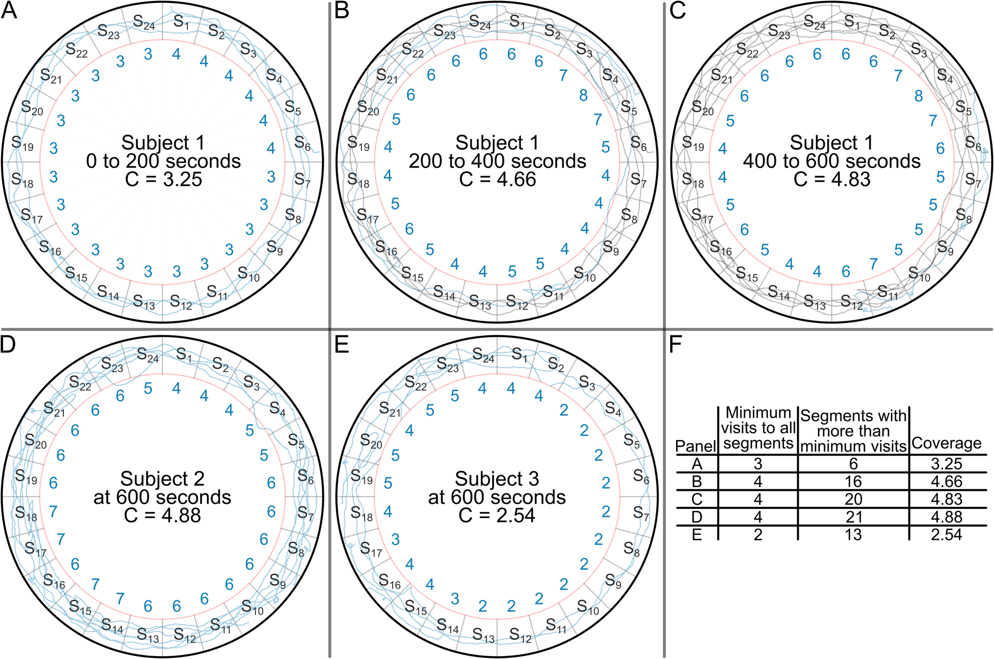
Coverage, a metric developed to mitigate the arena-size-dependency inherent in activity, is introduced as a novelty-based measure of exploration. In opynfield, we employ a sector-based approach to calculate coverage, dividing the arena area into sectors and counting visits to each sector. Visits are not merely the number of recording points located inside each sector. An animal may linger in one sector for an extended period, but this still constitutes one visit. On the other hand, depending on the sampling frequency and sector size, an animal may not be recorded inside a sector that it necessarily would have passed through to travel between the sectors it was recorded in. The function locate_bins identifies the number of visits made to each bin over time, which the function calculate_coverage uses to compute the final measure as defined in Eq. 3. This equation shows how coverage (C) can be calculated at each time point (t) from the number of visits made to each sector by that time point. Here, vmin(t) is the minimum number of visits made to any sector, such that all sectors at that time point have received a number of visits greater than or equal to vmin(t). M represents the total number of sectors, so that the sum from i to M is iterating over all sectors. χ is the indicator function where χ[x] = . v(i,t) is the number of visits made to sector i at time t. Thus, the argument v(i,t) – vmin(t) is greater than 0 when sector i has received more visits than vmin at time t. In total, the summation counts the number of sectors that have received more than vmin visits, and this is divided by the total number of sectors, M. Thus, coverage is essentially the number of visits that every sector has received plus the fraction of sectors that have been visited more times than that. This calculation is further illustrated graphically (Fig. 1).

Fig. 1

Prototypical examples of coverage. Throughout the course of an open field experiment, the subject explores the arena boundary. After dividing the arena into sectors (S1 to S24), we can count the number of visits made to each sector of the arena boundary and use the number of visits to calculate coverage. Each subject accumulates coverage over time. (a) A hypothetical subject, Subject 1, is tracked (blue trace) over the first 200 s of an experiment. The subject is first detected in sector 6 and makes three complete laps around the arena. Additionally, it travels from S6 to S1, making 4 total visits to those sectors. Thus, at t = 200 s, Subject 1 has vmin = 3, with 6 out of 24 sectors receiving more than vmin visits at that time. (b) The experiment continues to t = 400 s, and the subject makes more visits to each sector. The subject makes an additional complete lap, but doubles back several times, so that some sectors accumulate more visits than others. The number of visits made to each sector includes the visits accounted for previously (t = 0 to 200 s, gray trace), and the new visits made (t = 200 to 400 s, blue trace), which are considered together to count the number of visits to each sector. Then, coverage at t = 400 s is calculated from vmin = 4, with 16/24 sectors receiving more than vmin visits. (c) The experiment continues until t = 600 s, and the subject travels from S5 to S12, doubling back several times. Previous visits (t = 0 to 400 s, gray trace) and new visits (t = 400 to 600 s, blue trace) are considered together to count the total number of visits made to each sector. Coverage at t = 600 s is calculated from vmin = 4, with 20/24 sectors receiving more than vmin visits. When we calculate coverage at a finer timescale (typically every second, rather than every 200 s) and with more sectors (typically 3600, rather than 24), we can plot a nearly continuous function of how coverage accumulates over time. In addition to looking at how coverage accumulates over time within a given subject, we can also compare the total amount of coverage different subjects achieve throughout the course of an experiment. For example, Subject 2 (d) visits every sector at least 4 times, and visits 21 sectors more than 4 times, achieving a final coverage of 4.88. On the other hand, Subject 3 (e) only visits every sector at least 2 times, and visits 13 sectors more than 2 times, achieving a final coverage of 2.54. Thus, subject 2 requires approximately 2 × more learning opportunities to habituate to the novelty of the arena boundary than subject 3 does. If subjects 2 and 3 were part of the same experiment, this may represent genetic differences or effects of treatments. However, if they were run at different times, as a part of different experiments, it may represent differences in environmental conditions that influence the habituation processes, such as time of day or light levels. In panels a-e, blue numbers represent the number of visits made to the nearest sector. (f) These visits are used to calculate coverage by counting the minimum number of visits and the number of sectors with more than the minimum visits

$$C\left(t\right)=_}(t)+\frac\sum_^\chi [v\left(i,t\right)-_(t)])$$

(3)

For edge-dwelling animals such as Drosophila species, visits are only counted when they occur within a certain distance of the arena’s edge. This distance is controlled by the UserInput parameter, edge_dist_cm. The size of the sectors is defined by the Defaults parameter node_size, which determines the sector’s central angle in degrees, which must divide evenly into 360° to have equally sized sectors. While coverage is robust to changes in node_size, care should be taken to ensure the value results in sector arc lengths that make sense for the study subject (i.e., not orders of magnitude more or less than the subject’s body length). Because of these considerations, Cartesian coordinates (x and y) are converted to polar coordinates (r and theta), using the function cartesian_to_polar.

Coverage accurately measures the number of visits to each sector that an animal needs to learn or habituate to the novelty of that area. However, using raw coverage to examine activity or some other behavioral measure as a function of learning has limitations. The number of visits does not directly impact activity, but rather how much of the novelty habituation has been achieved by that time; when the animal has fully familiarized itself with its environment, it ceases specific exploration. Thus, opynfield calculates several re-scalings of coverage to use learning as a predictor of behavior. These alternative measures include percent coverage, percent of individual coverage asymptote (PICA), and percent of group coverage asymptote (PGCA).

Percent coverage simply takes an individual’s coverage vector and divides every value by the maximum coverage achieved during the recording. This normalization rescales the measure to be between 0 and 1, where the percent coverage value represents what fraction of novelty habituation has occurred. Percent coverage works well as a predictor of other behavioral measures when the animal reaches or nearly reaches the coverage required for full learning of the arena during recording.

If the recording time is too short for the animal to reach the coverage required to fully learn the arena (i.e., the time versus coverage relationship shows coverage is still increasing quickly and not reaching an asymptote), then the maximum coverage achieved during the recording is not a good measure of the animal’s coverage needed for full learning. Instead, PICA or PGCA may be more appropriate. In these cases, the coverage vector is rescaled by the predicted asymptote of the time versus coverage relationship. For PICA, the asymptote is calculated for each individual, while for PGCA, the group’s average coverage asymptote is used.

The functions calculate_percent_coverage and calculate_pica are used to calculate their respective measures as each Track is addressed. PGCA cannot be calculated until all Track objects have been converted to StandardTrack objects, at which point tracks_to_measures groups them by experimental group and calculates the group coverage asymptote with calculate_group_coverage_asymptote. At this point, the PGCA for each StandardTrack is calculated with calculate_pgca.

The module culminates with the computation of motion probabilities, which measure the directional persistence of test subjects. These probabilities, including P++, P+-, P+0, P0+, and P00 (Eqs. 4–8), evaluate the likelihood of specific turns or decisions between consecutive steps (Fig. 2). By accounting for directional changes, these probabilities contribute to a more nuanced understanding of exploratory drive and how it differs from random motion in the arena. These measures are calculated for a population rather than for individuals.

Fig. 2

Prototypical examples of directional persistence behaviors. Throughout the course of an open field experiment, the subject explores the arena boundary. The overall exploratory path (a) can be broken down into step-by-step decisions. At the beginning of an experiment (red box, panel a), Drosophila exhibit high directional persistence. (b) Following a step forward from point P1 at time t1 to P2 at t2, the subject’s next step can be classified into three categories. (c) The subject can take another step in the same direction (❘ϴ❘ ≤ 90°) to P3 at t3, contributing to P++. (d) The subject can take a step in the reverse direction (❘ϴ❘ > 90°) to P3 at t3, contributing to P+-. (e) The subject can stop and remain at P2 until t3, contributing to P+0. (f) Later in an experiment (blue box, panel a), Drosophila exhibit less directional persistence and more rest. Following a rest, where the subject remains at P1 from t1 to t2, the subject’s next step can be classified into two categories. (g) The subject can stay at P1 until t3, contributing to P00. (h) The subject can take a step in any direction to P2 at t3, contributing to P0+

$$_\left(n\right)=Prob(\Delta _>0|\Delta _>0)$$

(4)

$$_\left(n\right)=Prob(\Delta _<0|\Delta _>0)$$

(5)

$$_\left(n\right)=Prob(\Delta _=0|\Delta _>0)$$

(6)

$$_\left(n\right)=Prob(\Delta _>0|\Delta _=0)$$

(7)

$$_\left(n\right)=Prob(\Delta _=0|\Delta _=0)$$

(8)

In these equations, the sign of ΔD is taken relative to the previous step. This means that the motion probabilities are calculated based on the angle between two consecutive steps (three consecutive tracking points). When the magnitude of an angle is less than 90°, that turn is considered positive or in the same direction as the previous step, while a turn with an angle greater than 90° is considered negative or in the opposite direction as the previous step. Undefined turns occur when one or both steps have a ΔD = 0, in which case P+0, P0+, and P00 are determined by step length alone. Since the motion probabilities are contingent on their initial condition being met (a step occurring for P++, P+-, and P+0, or a rest occurring for P0+ and P00), some motion probabilities will be very rare to observe, especially P00. The function turning_angle uses the law of cosines to determine the angle between consecutive steps. These angles are taken together with activity to compute the motion probabilities. Note that for n coordinates, there are n-1 steps and n-2 turns or decisions. A decision or turn taken at time i occurs between step i-1 (time i-1 to i) and step i (time i to i + 1). Additionally, calculation shortcuts can be made due to the relationships among the motion probabilities given in Eqs. 9 and 10.

The function motion_probabilities first determines what type of turn or decision was made by each individual, generating an array of ones and zeros for each measure. Taking P++ as an example, a one in this array would mean that at that time point, the animal had just completed a step and was initiating a step in approximately the same direction, while a zero would mean it either had not completed a previous step (was at rest; P0+ or P00), or did complete a step, but was initiating a step in the opposite direction (P+-) or was initiating a rest (P+0). Next, the group’s motion probabilities are calculated with motion_probabilities_given_previous. For example, P00 at time i is the number of individuals with a 1 in their individual P00 array at time i, divided by the number of individuals with a 1 in either their P00 or P0+ array at time i. Thus, we set up an array with 1 where P00 occurred, 0 where P00 could have occurred but didn’t (i.e., P0+ occurred), and NaN elsewhere.

These measures may apply differently in other study organisms, so two additional versions were developed. The original version of the motion probabilities described above is designated motion probabilities given previous (e.g., P+-Given+) elsewhere in the documentation to differentiate it from motion probabilities given any and raw motion probabilities. Motion probabilities given any (e.g., P0+GivenAny) are calculated similarly. For example, this P00 at time point i is the number of individuals that had a 1 in their P00 array at time i, divided by the number of individuals that had a 1 in their P++, P+-, P+0, P0+, or P00 array at time i. In this case, Eqs. 4, 5, 6, 7, 8, 9 and 10 do not hold, but instead the relationship is found in Eq. 11. This differs from raw motion probabilities because all versions of motion probabilities are calculated only in the edge region. This means that the sum of individuals that had a 1 in their P++, P+-, P+0, P0+, or P00 array at time i is not necessarily the total number of individuals in the group. Raw P++ would be calculated with the number of individuals in the group in the denominator.

Module 4: Behavioral Measure Summary

Once these exploration metrics are calculated, the behavioral measure summary module (summarize_measures) synthesizes the individuals’ data into group-level insights. Additionally, the module produces outputs that can be used for external analysis.

The initial step in this module involves the individual_measures_to_dfs function, which compiles individual behavioral measures for each group into CSV files. Next, the module employs the function all_group_averages to calculate each relationship's group-level average and standard error of the mean (SEM). Group calculations are straightforward for temporal relationships, such as computing the mean activity at each time point, since all tracks are measured with the same sampling frequency. However, complexities arise for predictors like cover. For example, plotting average coverage against average activity would fail to capture the relationship seen in the individuals. Instead, this approach would show the average activity and coverage at a certain time point rather than the average activity at a certain coverage level. To address this, opynfield reverts to raw data for measures involving coverage. Tuples of coverage-activity pairs from all individuals in a group are aggregated, and the average activity values at specific coverage points are computed. To handle the continuous nature of coverage, bins or ranges of coverage values are introduced to group these tuples to be averaged. These bins are determined either by the number of tuples they contain (n_points) or by a set range size (n_bins). The n_points method performs better and is employed for coverage, PICA, and PGCA, while the n_bins method performs better and is used for percent coverage. Once each temporal and coverage-based relationship is summarized, a CSV file is produced for the average and SEM of each group.

Module 5: Model Fitting

The model fitting module (fit_models) is used to reveal the relationships between exploratory measures at individual and group scales. The module calculates the parameters that optimally characterize these relationships, employing the functions specified in the earlier ModelSpecification objects. For instance, the time versus activity relationship in Drosophila species takes the form of an exponential decay (Eq. 12), where a, b, and c are parameters that govern different facets of the exploration process. The exponential decay form aligns with the observed behavior of Drosophila species, where activity starts at elevated levels and decreases asymptotically.

Due to the potential presence of outliers, opynfield employs a robust strategy to prevent the undue influence of outliers on the analysis. Instead of outright exclusion, which could potentially remove most of the data due to the large number of relationships being analyzed, the module employs parameter bounds based on the distribution of parameters observed among individuals in the same group during the naïve fit. The function fit_all performs the naïve fit, after which find_fit_bounds establishes parameter ranges, which span two standard deviations below to two standard deviations above the mean of each parameter. This bound-setting approach is modifiable through the optional UserInput parameter bound_level and provides a balanced means to address outliers without discarding useful data.

After the computation of parameter bounds, opynfield employs the re_fit_all function, which integrates these constraints to calculate the new best-fit parameters. The resultant values are exported as a CSV file for further analysis via the format_params function. These formatted individual parameters also set the stage for opynfield’s in-house statistical analyses.

In addition to the best-fit parameters for each individual, the group-level model parameters may also be of interest. The function group_fit_all leverages the previously calculated parameter bounds from individual fits and applies them to the model fitting process using the group-averaged data. The ensuing group parameters are formatted for future analysis by format_group_params and exported into CSV files.

Model Choice

Due to the diversity of study organisms and experimental contexts that open field exploration can address, opynfield accommodates flexibility in the functional forms employed for model fitting. Table 1 outlines the six functional forms used in the sample analyses. The default ModelSpecification settings use the exponential decay model (Eq. 12) for activity, P++, and P+0, and the asymptotic increase model (Eq. 1) for coverage, P+-, P+0, and P00. Users can select a different pre-defined function based on known patterns of exploration or patterns observed in their data. For example, in the fourth sample analysis, we edit the ModelSpecification object to use linear models for the motion probabilities. Additionally, users can create a data class to specify a user-defined functional form. This is demonstrated in the first sample analysis, where we create the sigmoidal decay and sigmoidal increase data classes to be used for the motion probabilities. This flexibility allows users to tailor their analyses to their specific research requirements.

Table 1 Standard function options for model fitting

While maintaining flexibility in function specification, the default functions embedded in opynfield’s model fitting module, as well as those used in the sample analyses, boast high interpretability. Taking the time versus activity relationship as an example, parameters a, b, and c individually influence distinct aspects of exploration. Differences in these parameter values offer insights into the underlying processes of initial activity/neophilia (parameter a), habituation speed (parameter b), and steady-state activity levels (parameter c), respectively.

Module 6: Statistical Tests

In order to leverage the interpretability of the model parameters, the next module (stat_test) performs statistical tests directly on the individuals’ best-fit parameters. The primary statistical tool used in opynfield is the Multiple Analysis of Variance (MANOVA) test. In this test, each parameter derived from the model fits assumes the role of a dependent variable, while the experimental groups act as the independent variable. This approach allows for a holistic assessment of group-level variations in behavior. Given the substantial number of tests conducted, executing a full MANOVA model demands considerable data. Thus, opynfield also introduces the concept of "sub-tests." These sub-tests are MANOVA analyses on all parameters associated with a specific relationship, offering a pragmatic alternative for scenarios with limited data availability. By default, opynfield fits models for all versions of the motion probabilities and models each variable by time as well as by each version of coverage. Thus, sub-tests are also useful when you are only interested in a subset of these relationships, such as using only the “given previous” versions of the motion probabilities and using only percent coverage as an independent variable.

Following a statistically significant MANOVA (or MANOVA sub-test), the Analysis of Variance (ANOVA) test is applied to each parameter that was included in the MANOVA. Here, the parameter functions as the dependent variable, and, once again, the experimental group constitutes the independent variable. The ANOVA tests pinpoint specific parameters that contribute significantly to observed differences.

In the final stage of the statistical evaluation, pairwise t-tests are conducted on each parameter. This identifies specific groups exhibiting significant differences from one another and provides a nuanced understanding of behavioral variation. The execution of all tests is automated through the run_tests function, streamlining analysis.

The outcome of the MANOVA, ANOVA, and t-tests is documented in tables saved to a text file. For determining the significance of each test, users are directed to examine the Pr > F, PR(> F), or pvalue-hs columns, respectively. Additionally, the coef column of the pairwise t-test results should be used in conjunction with the exported model parameters to determine effect sizes and biological significance. Comprehensive details regarding the statistical tests, their output, and interpretations can be found in the package documentation.

Module 7: Plotting

The opynfield package culminates in the final module (plotting), which automates plot generation, allowing users to visualize the results derived from the preceding modules. The plotting module creates five distinct categories of plots, tailored to different stages of analysis.

First, the function plot_traces depicts the trajectory of the tracked organism alongside the inferred arena boundary. These plots may be useful early in the analysis to ensure accurate data reading, detect tracking errors, and identify anomalies in activity or arena boundary distortions.

Next, the function plot_all_individuals illustrates specific behavioral measure relationships for individual subjects. Customizable PlotSettings parameters can control the addition of model fit curves or equation layers. These plots can be used to validate the function chosen to model activity measures (e.g., determine if the activity exhibits an exponential decrease over time).

Additionally, the function plot_all_solo_groups reveals the average relationship between two variables for a specific group. Here, too, customizable PlotSettings parameters can control the inclusion of additional layers such as model fit curves, model equations, and SEM error bars on the average data points. This offers a collective view of the group dynamics.

The solo group plots are best utilized in conjunction with the group component plots generated by the function plot_components_of_solo_groups. These plots present the average relationship for a group alongside the raw data from all the individuals within that group. In addition to the solo group plot parameters, users can optionally specify the inclusion of individual model fits in the background using PlotSettings. These plots aid in choosing the optimal versions of coverage and the motion probabilities for a specific application and can verify that the group dynamics align with the individual-level trends.

Finally, the group comparison plots generated by plot_all_group_comparisons show the averages of all groups in the experiment. Users retain the same optional layers as in the solo group plots. These plots are used at the end of an experiment to visually highlight the differences between groups identified in the statistical test module.

Numerous PlotSetting parameters govern the generation and storage of plots. Detailed information on these parameters is available in the tutorial and documentation.

Availability

The opynfield package is a powerful tool for analyzing open field exploration tracking data and is readily accessible to researchers. The software is freely available on the Python Packaging Index (PyPI) or can be obtained directly from its GitHub repository (https://github.com/EllenMcMullen/opynfield).

The GitHub repository serves as a comprehensive hub, hosting the software package alongside resources to facilitate use. In addition to documentation, a tutorial is provided as a Jupyter notebook within the repository, allowing users to run analyses with the included test datasets. The tutorial guides users through core functions, enabling them to practice with curated data before adapting the workflow to their own datasets. The repository also features a user-support community, including a discussion board where users can pose questions to other users or the authors. This community resource assists both individual users and the broader group by addressing shared challenges and questions. It also serves as a conduit for feature requests, allowing users to suggest additions or modifications to help ensure that opynfield evolves in line with user needs.

The package utilizes several other open-source packages, including pandas (The Pandas Development Team, 2023), scipy (Virtanen et al., 2020), numba (Lam et al., 2015), statsmodels (Seabold & Perktold, 2010), and matplotlib (Hunter, 2007). Full dependency information can be found in the supplementary materials (Online Resource 1). opynfield is available under the GPL-3.0 license. The version used in this paper is archived on Zenodo (https://doi.org/10.5281/zenodo.15794680). For further information on installation and usage, see Online Resource 2.