As early as 1875, researchers have recorded electrical signals from living mammalian brains [1]. Fifty years later, in the 1920s, researchers began to record electroencephalography (EEG) from the human scalp, sparking decades of investigation and debate regarding the source of this signal [2]. By the 1970s experimental neurobiologists, theoretical biophysicists, clinical researchers, and electrical engineers were all actively contributing to the burgeoning field of EEG source analysis [3–7]. Theories emerged regarding a dipole model of EEG sources, where intracellular and extracellular flow of ions in pyramidal neurons create dipolar charges large enough to be measured at a distance [8]. However, the realities of winding gyri and sulci beneath heterogeneously conductive cranial bone present additional challenges to the already ill-posed problem of source estimation from EEG [9]. Regardless, it became clear that the EEG system of electrical sensors recording from the scalp, despite its challenges, offered a promising method to noninvasively infer underlying neurophysiological activity.

In the hundred years following this early pioneering work, researchers and clinicians have found numerous uses of the EEG signal. These uses include guiding neurologists and neurosurgeons to treat epilepsy, providing anesthesiologists measures of consciousness, assisting somnologists in sleep stage analysis, and offering cognitive scientists a glimpse into the stereotyped activity relating to perception and language processing [10–13]. The EEG signal has also been explored as a biomarker for numerous conditions, including depression, mild traumatic brain injury, and dementia [14–16]. At the same time, advances in techniques for source estimation from EEG have allowed for improved spatial resolution, scientific discovery, and clinical applications [17]. The development of high-density EEG (hd-EEG), which employs 64 or more channels, has helped overcome the spatial resolution limitations of standard EEG systems and improve the performance of source localization methods [18, 19]. EEG remains a popular choice for the development of noninvasive neurophysiological biomarkers and brain-computer interfaces due to its relatively low-cost and portable nature [20].

However, EEG is not the only modality for measuring neural activity. Invasive approaches such as stereotactic EEG (sEEG) involve the implantation of depth electrodes, enabling the recording of electrical activity closer to the sources. Other noninvasive alternatives leverage magnetic techniques to image neural activity, which often require cryogenic cooling and shielded environments, limiting their portability. Magnetoencephalography (MEG), for example, detects the magnetic fields generated by currents in the skull, offering a complementary signal to EEG due to the orthogonal orientation of the electric and magnetic field components. Other modalities contribute by modeling the biophysical structure of the subject’s head or by inferring neural activity indirectly through changes in blood flow and oxygenation, which are believed to reflect underlying neuronal activation. Magnetic resonance imaging (MRI), for example, although primarily used for structural imaging to help biophysical modeling of cranial geometries, can also capture functional activity of neural sources through techniques such as functional MRI (fMRI). Each modality offers distinct advantages and limitations in terms of spatial resolution, temporal resolution, invasiveness, and portability, but none of the methods are as portable or economical as EEG.

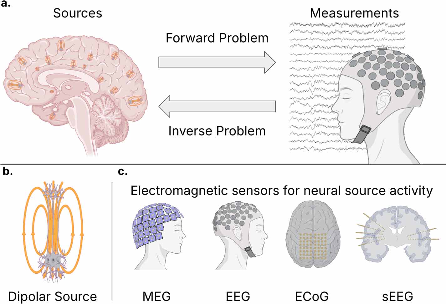
This topical review synthesizes neural source estimation and localization techniques emphasizing EEG-based approaches. We begin by reviewing the background on neural sources and modalities to measure these sources before summarizing models that solve the forward problem of propagating source activity to sensor measurement recordings. We then review existing models to solve the inverse problem of estimating source activity from the sensor measurements. An illustration of the forward and inverse problem of neural source estimation and electromagnetic recording modalities is shown in figure 1. The review includes a summary of state-of-the-art methods, including techniques that model nonlinearities, scale to higher-density EEG recording systems, and leverage multiple modalities. Additionally, we discuss extensions of source estimations, such as estimating invasive measurements from noninvasive measurements. This discussion includes a summary of the key challenges remaining in neurophysiological source estimation. After reviewing techniques for source estimation, we synthesize the clinical uses of neural source estimation in practice today and potential future applications of neural source estimation and review the existing software and data available for researchers and clinicians to estimate source activity from EEG data. Finally, we propose a strategic roadmap for the field, outlining concrete milestones across varied time horizons to continue improving neural source estimation techniques. This work aims to offer a summary of the state-of-the-art techniques and challenges in neural source estimation, extending beyond linear inverse problem modeling on standard EEG systems.

Figure 1. Overview of the forward and inverse problems in neural source estimation and associated recording modalities. (a) Schematic representation of the relationship between neural activity and sensor data. Here, the forward problem models how electromagnetic fields generated by distributed neuronal sources propagate through head tissues to be recorded as measurements at the sensors, and the inverse problem leverages these sensor measurements to estimate the location, orientation, and amplitude of the underlying sources in the brain, which may be time-varying. (b) Illustration of the dipolar model of neuronal activity, where ensembles of pyramidal neurons form equivalent dipole moments due to the flow of ions across the length of the cell. (c) Common electromagnetic sensing modalities used to record neural activity. These include noninvasive methods, such as magnetoencephalography (MEG) and electroencephalography (EEG), and invasive intracranial methods, including electrocorticography (ECoG) placed on the cortical surface and stereoelectroencephalography (sEEG) using penetrating depth electrodes.

Download figure:

Standard image High-resolution image 2.1. What are neural sources?

From a signal processing perspective, sources refer to the generators of signals. In other words, a source is the origin of information. In the context of the brain, the nature of neural sources has been debated [21, 22].

The dipole theory is a biophysical theory that relies on fundamental electromagnetic physics and volume conduction for the neuronal source to be measurable at a distance. The cellular origin of these dipolar sources is widely attributed to pyramidal neurons [23], whose aligned geometry and orientation within the cortex facilitate the summation of extracellular potentials and allow for spatially distributed current flows rather than a simple imbalance of charge. During synaptic activation, ionic flow into the cell at the distal dendrites and exit via other parts such as the soma or basal dendrites, creating a separation of charge and forming postsynaptic transmembrane currents [24]. As a result, the dipole theory of neurological sources models current sources or sinks within neuronal tissue via equivalent current dipole moments (illustrated in figure 1(b)), which are measured in Ampere-meters (A-m). The current of a single pyramidal neuron’s postsynaptic potential is typically modeled to be on the order of 20 fA·m, which suggests that evoked potentials observed in scalp recordings on the order of 10 nA·m comprise millions of synapses [25]. Biophysicists continue to add detail to this equivalent dipole model of neural sources, accounting for action potential quadrupoles, reversal potential, and presynaptic activity [26–28].

More detailed theories of neural sources expand beyond the notion of simple localized dipoles measurable at a distance via volume conduction. Simpler models of brain sources assume a limited number of dipoles in fixed locations, while more realistic models seek to estimate current sources distributed throughout the brain [29, 30]. Additionally, some neurophysiologists have preferred to view sources of measurable electrical brain activity as the result of cortical field potentials modulated by interactions with tissue [31]. The interaction of electrophysiological activity with tissue poses numerous challenges to the estimation of source activity. Volume conduction of the electrical activity along conductive pathways implicates changing dielectric properties of the brain tissue, cerebral fluids, and cranial bone [32–34]. Researchers in 2009 summarized 4 working source activity models: the equivalent-current dipole model, dipolar models in overdetermined problems, the cortical model, and the potential distribution inside the head [35]. The equivalent-current dipole model referred to the assumption of a single macro dipole, and the dipolar models in overdetermined problems referred to the models considering a small number of sources. The cortical model assumed no contribution of deep sources, while the potential distribution model generalizes across these models without making claims regarding the origins of these potential sources. Since that time, researchers have converged upon the distributed potentials resulting from micro and macro current sources and sinks forming dipoles or higher order n-poles [8, 36]. Additionally, research indicates that subcortical activity influences electrophysiological recordings of brain activity, especially with high density EEG [37] or MEG [38].

For many engineers and clinicians, the exact nature of neural sources is secondary to its utility as an underlying signal that can cause or explain neurological or psychiatric function and dysfunction. From the engineering perspective, the problem of estimating sources across the brain is underdetermined with multiple potential solutions, so biological, physical, or application-driven constraints are necessary to find purported sources of activity. As a result, researchers often take data-driven approaches, making use of functional connectivity and biophysical assumptions to estimate sources [39, 40]. Clinicians, especially in epilepsy monitoring units, focus on identifying functional regions, such as the epileptogenic zone and eloquent cortex [41, 42]. From these practical perspectives, the benefits of source estimation techniques are their ability to explain and treat neurophysiological function and dysfunction.

2.2. How are sources measured?

Neural source activity is measured via two main categories: direct electromagnetic recordings and indirect hemodynamic measurements. Electromagnetic methods offer high temporal resolution, while hemodynamic methods may provide greater spatial resolution, with ongoing efforts to integrate modalities. In the following sections, we offer a brief overview of the modalities available to infer neural source activity and highlight active areas of research focused on integrating multiple modalities.

2.3. Direct electromagnetic recodings2.3.1. Electroencephalography

EEG measures brain electrical activity as voltage differences between an electrode and a reference. Scalp EEG uses a standardized array to record scalp voltages against a non-neuronal reference, such as the mastoid bones or earlobe. Computational processing allows re-referencing and algorithms to estimate scalp-measurable source potentials. Source estimation algorithms may assume fixed [43, 44] or distributed sources [45, 46]. Key challenges include noise (e.g. motion artifacts, electromagnetic interference, heterogeneous propagation) and limited spatiotemporal resolution (depth and cortical). hd-EEG arrays improve spatial resolution [18, 19]. Approaches addressing these limitations include incorporating individual morphology via multimodal imaging [47, 48] and using complementary modalities like MEG and functional near-infrared spectroscopy (fNIRS) to improve source estimation quality and efficiency [49–53]. For reviews on the history and applications of EEG source localization, see [2, 14, 30, 54, 55].

2.3.2. sEEG

sEEG measures extracellular electric potential inside the brain via neurosurgically inserted penetrating depth electrodes. This provides voltage measurements closer to the source, reducing attenuation and noise compared to scalp EEG. However, the procedure is invasive, requiring specialized neurosurgeons and equipment [56]. While a meta-analysis found complication rates of 0.9%–1.7% [57], a recent large cohort study reported zero complications [58]. The heterogeneous and subject-specific spatial distribution of sEEG contacts complicates inverse modeling and algorithm generalization, requiring precise morphological and contact locations to be accounted for [59]. Automated or semi-automated frameworks using pre-surgical MRI and post-implantation CT scans help localize these contacts [60–63]. The sEEG recordings serve as a complementary modality for data-driven scalp EEG source localization techniques [64–66]. Due to its invasive nature, sEEG is clinically restricted (e.g. drug-resistant epilepsy) and infeasible for source estimation in most populations [67]. Nonetheless, intracranial clinical and animal recordings offer a valuable research resource and potential training signal for source estimation models, and there is active research in identifying the shared information between scalp and intracranial EEG (iEEG) [68–70].

2.3.3. Electrocorticography (ECoG)

ECoG, another form of iEEG, involves electrodes placed beneath the skull on the cortex surface, either subdurally or epidurally [71]. Used clinically since 1939, ECoG monitors epileptiform activity and guides resection surgery, especially for superficial regions [72, 73], and is also used to study network dysfunction in Parkinson’s disease [74, 75]. Many centers now prefer sEEG because it is less invasive, samples 3D cortical/subcortical structures, and has lower complication rates (e.g. hemorrhage, infection) [76]. ECoG (like sEEG) offers high temporal/spatial fidelity, avoiding skull-induced signal attenuation, but lacks sEEG’s 3D spatial coverage [77]. Several studies have demonstrated that incorporating ECoG signals into inverse modeling pipelines can improve source localization accuracy, especially when used to constrain or validate solutions [77–79]. As a result, similar benefits may be obtained by using sEEG data to constrain noninvasive source estimation techniques.

2.3.4. Magnetoencephalography

MEG records neural activity from brain electrical currents using magnetometers to measure magnetic field changes and gradiometers to measure their spatial gradients. As a result, MEG measures aspects of the source electromagnetic field complementary to EEG. Magnetic fields generated by neural currents are also less sensitive to tissue and bone attenuation than electric field potentials. However, the interface between tissues of differing conductivities, such as the skull [80] cerebrospinal fluid (CSF) [81], can alter the distribution of secondary volumetric currents, which influence the measured field. This technology was first enabled by superconducting quantum interference devices, which require significant amounts of cooling that limits their portability [82]. In recent years, researchers have developed more portable magnetometers that function at ambient temperatures. These technologies include the spin-exchange-relaxation-free (SERF) optically pumped magnetometer (OPM) [83] and the magnetic-field-modulation-free OPM [84], the latter achieving broader bandwidth than the SERF OPM. Further advances in MEG portability will help expand its utility in source localization and estimation. We direct the reader to [25, 85] for further reading on MEG source estimation.

2.4. Functional hemodynamic measurements

MEG, along with scalp, stereo, and iEEG are the primary means to directly measure source electrical activity. However, several modalities measure the hemodynamic response, which is believed to correspond to source activity [86]. Although these measurements do not directly measure dipolar sources, functional measures of source activity have shown promise in localizing and estimating cortical and subcortical activity. Additionally, functional and indirect measurements have shown a complementary role in source estimation by capturing neurophysiological dynamics.

2.4.1. fMRI

MRI uses magnetic fields and radio pulses to generate images of tissue. Structural MRI provides 3D brain images with resolutions from ∼0.2 mm at 11.7 T, to 0.5 mm at 7 T, and 1–2 mm at 3 T [87–90]. These high-resolution images can help constrain subject-specific biophysical source modeling and localize intracranial recording contacts. fMRI infers neuronal activity from blood-oxygen-level-dependent changes in blood flow [91]. While this method is noninvasive and offers strong spatial resolution, the temporal resolution is limited to seconds. Although some studies have reached sub-second sampling rates [92, 93], the seconds-long biological timescale of the hemodynamic response [94] remains a limiting factor for further technical advances. MRI systems usually require large, cooled magnets, but low-field portable scanners are emerging [95–97]. Multimodal integration of fMRI with EEG has shown improved source localization spatial resolution [48, 98, 99]. However, EEG systems are not always MRI compatible, and MRI compatible EEG signals are typically contaminated with artifacts despite ongoing artifact reduction efforts [100]. When feasible, fMRI remains a useful concurrent modality for estimating source activity.

2.4.2. fNIRS

fNIRS uses the absorption of near-infrared light by oxygenated and deoxygenated hemoglobin to estimate hemodynamic activity. Since its first single-channel recordings in 1992, fNIRS has developed into multichannel systems capable of three-dimensional tomographic reconstructions [101]. High-density diffuse optical tomography (HD-DOT) helps extend the limited field of view, but imaging sensitivity remains limited beyond 1.5–2 cm beneath the skull [102]. Techniques such as confocal time-of-flight DOT have been shown to improve the resolution to millimeter scales [103]. The 2–10 Hz temporal resolution of fNIRS is faster than fMRI but slower than EEG [104]. As with fMRI, the biological timescale of the hemodynamic response constrains fNIRS analysis. Integrating fNIRS with electrical modalities, such as EEG, may offer complementary information that enhances functional network modeling and helps localize pathological source regions, including the epileptogenic zone [105–107]. Given its potential as a portable, noninvasive complement to scalp EEG, further research on synchronous EEG-fNIRS recordings for source estimation is needed.

2.4.3. Other hemodynamic imaging modalities

While fNIRS and fMRI are the most commonly used noninvasive methods for measuring brain activity besides EEG, several other modalities are worth mentioning due to their role as complementary modalities. For example, emission tomography such as positron emission tomography (PET) and single-photon emission computed tomography (SPECT) use radiotracers to measure cerebrovascular activity [108]. These methods have limited spatial resolution or source estimation capability on their own, but demonstrate improved ability to determine diagnostic outcomes when combined with EEG source imaging [109, 110], although the expensive and non-portable nature of emission tomography limit their widespread use.

Other modalities remain in earlier stages of development for functional source imaging. Functional ultrasound (fUS) leverages the Doppler effect and ultrasound waves to image fluid flow. While this method is useful for measuring blood flow velocity in major arteries, it has also been used to image neuronal hemodynamic responses in humans [111, 112] and efforts are underway to integrate EEG with fUS [113]. Photoacoustic tomography (PAT) is an emerging technology that also leverages ultrasonic principles by pulsing laser light which is absorbed by the tissue and causes thermoelastic expansion that generates ultrasound waves [114]. PAT achieves greater penetration depth for imaging than fNIRS [115] and has been used to measure BOLD signal in humans [116], but further work is needed to determine proper molecular targets [117] and develop algorithms that incorporate EEG and estimate source activity. Another promising noninvasive modality is electromagnetic wave-based imaging (EMI). Gigahertz frequency waves have been used to estimate varying dielectric properties of tissue, including the brain [118–120], where researchers are investigating the detection and localization of stroke [121, 122]. Because the dielectric properties are expected to change not only with changes in blood flow but with ionic concentration changes caused by action potentials, there are efforts to estimate neuronal firing with EMI [123, 124], but further work is needed to ensure the focality of the measurement and maintain specific absorption radiation rates within the safe limits.

To improve source EEG and MEG localization and estimation, promising complementary modalities could help determine conductivity for personalized modeling. Electrical impedance tomography (EIT), for example measures tissue conductivity using small currents and can track intracranial conductivity changes related to blood flow and pressure [125, 126]. It has clinical applications [127, 128], complements EEG/MEG with patient-specific conductivity models [129], and can even image neuronal activity at high spatiotemporal resolution in peripheral nerves [130, 131]. Integrating EIT with OPMs is an emerging approach for fast, noninvasive source imaging [132]. An even more nascent conductivity measuring method is magnetoacoustic tomography (MAT), where a time-varying external magnetic field generates acoustic fields which can estimate the conductivity distribution of tissue [133]. Research efforts continue to be made to develop MAT systems and characterize their biophysical responses, especially as a technique for electrical impedance imaging [134, 135]. Modalities that measure head conductivity need more research to validate their measurements and to build models that can properly use that data.

These modalities each represent promising directions for noninvasive imaging of neural activity, but further work is needed to develop the methodologies, validate their biological interpretation, and integrate these techniques with modalities, such as EEG and MEG, that directly measure electrical activity in the brain.

A core challenge in neural source analysis is accurately modeling the forward propagation of source activity to scalp sensor measurements. This section reviews established approaches to the forward problem, from simplified models to more advanced methods that account for individual anatomical variability, and highlights promising directions for improving both model accuracy and computational efficiency. In EEG source analysis, the forward problem plays two key roles: it provides a biophysically grounded framework for validating source estimates and enables the generation of realistic simulations of brain activity and corresponding EEG data.

More broadly, estimating neural source activity typically involves three major steps: 1. modeling neural electrical activity, 2. modeling head volume conduction to relate neural sources to scalp potentials (the EEG forward problem), and 3. reconstructing source activity from EEG measurements (the inverse problem) [136, 137]. The forward problem predicts electric field measurements on the scalp given source configurations, while the inverse problem attempts to estimate the sources that gave rise to the recorded signals. The forward problem can be described as finding function (1), while the inverse problem seeks the function f (2). Here, denotes the time-varying source signal across p locations and T time steps while denotes the signal measurements across Nm sensors or channels. Typically, Nm is between 16 and 32 channels for standard EEG or 128–256 for high density EEG, although there is evidence that as few as 6 channels may be capable of estimating a single source [138] and ultra high density EEG systems with 1024 channels are an active area of research [139],

The accuracy of the forward model directly influences the precision of source localization and therefore plays a critical role in solving the EEG inverse problem. Traditional EEG forward models typically assume linearity, static conductivity, and isotropic tissue properties, simplifications that limit the physiological realism of the solutions [136]. Recent studies highlight the importance of incorporating more accurate, nonlinear forward models that capture biophysical complexity and individual anatomical variability, including morphological variation caused by developmental or pathological changes [140–142]. In this section, we approach the EEG forward problem by first reviewing models of neural electrical activity, including a mathematical framework, followed by an overview of the most commonly used head volume conduction models.

3.1. Neural mass models ((NMMs) and generative models of EEG

While foundational models like the Hodgkin–Huxley formalism established the mathematics of single-neuron membrane dynamics [143], these microscopic descriptions do not scale to macroscopic neuroimaging. The Wilson–Cowan model bridged this gap by formally describing the activity of interacting neural populations [144]. However, interpreting EEG requires linking these population dynamics directly to the biophysics of signal generation, which the Jansen–Rit framework addressed by modeling the intrinsic connectivity between pyramidal cells and interneurons within a cortical column [145, 146]. Crucially, this connects mesoscopic dynamics to the EEG forward problem: the summed post-synaptic potentials of perpendicularly oriented pyramidal cells yield a time-varying equivalent current dipole. This dipole serves as the biophysical source for forward modeling of the scalp potentials, connecting neural mass equations to observable EEG signals.

3.2. Forward modeling: physical approximations

To mathematically solve for scalp potentials, the quasi-static approximation is applied, since the low-frequency nature of EEG renders displacement currents and wave propagation within the head volume negligible. In a linear ohmic medium, the electric field is proportional to the current density and satisfies , where is the electric scalar potential at location r. Charge conservation reduces Maxwell’s equations to the Poisson-type partial differential equation

where denotes spatially-varying conductivity and is the primary current density caused by source activity. Under the quasi-static approximation, (3) is linear in the source term. Consequently, the potential φ generated by a single dipole scales linearly with its dipole moment, and the contributions from multiple dipoles combine via electromagnetic superposition to produce the measurable scalp potentials.

Sensor-domain mapping. In practice, researchers evaluate (3) at discrete scalp sensor locations . A single current dipole is the primary current density evaluated at a singular point rq, with corresponding dipole moment q. The potential at sensor m is denoted for this dipole as

where, is the sensor-specific lead-field vector describing the linear relationship between the unit dipole and measured electrical potential. For clarity, we adopt a theoretical ‘infinite’ reference in this notation, while in practice, recordings use a physical reference; results stated under the ‘infinite’ reference can be re-referenced in the usual way without changing the underlying physics. For multiple dipoles indexed by k, by electromagnetic superposition, the potential is simply the sum

For convenience, we include table 1 describing the key mathematical notations used to synthesize the forward and inverse models.

Table 1. Summary of the notation used to describe the electromagnetic forward and inverse problems, including scalars, vectors, matrices, and functions.

SymbolType/dim.DescriptionSource amplitude matrixMeasurement data matrixNoise matrixNumber of sensors and sourcesForward-field matrix for multiple dipolesgFunctionForward mapping: fFunctionInverse mapping: Scalar electric potentialrSpatial position vectors (dipoles: rq, sensors: rm)Scalar or Electrical conductivity, isotropic or anisotropicDipole moment vector at time tDipole orientation (assumed normal to cortex)Sensor data vector at time tNoise vector at time tLead-field vector for dipole q and sensor mForward field vector for unit dipole at rq3.3. Head volume conduction models for EEG forward problem

Once neural electrical activity is modeled, typically using current dipole sources as described above, the next step in solving the EEG forward problem is to define a head volume conduction model. This model represents the conductive properties of head tissues and describes how electric currents propagate from neural sources through various tissue compartments to the scalp, enabling the computation of the resulting surface potentials.

Early approaches to EEG forward modeling employed simplified geometries, such as the homogeneous spherical head model, and later, multi-shell concentric spherical models, which allowed for analytical or semi-analytical solutions to the Poisson equation (3) governing electric potential distribution [147, 14