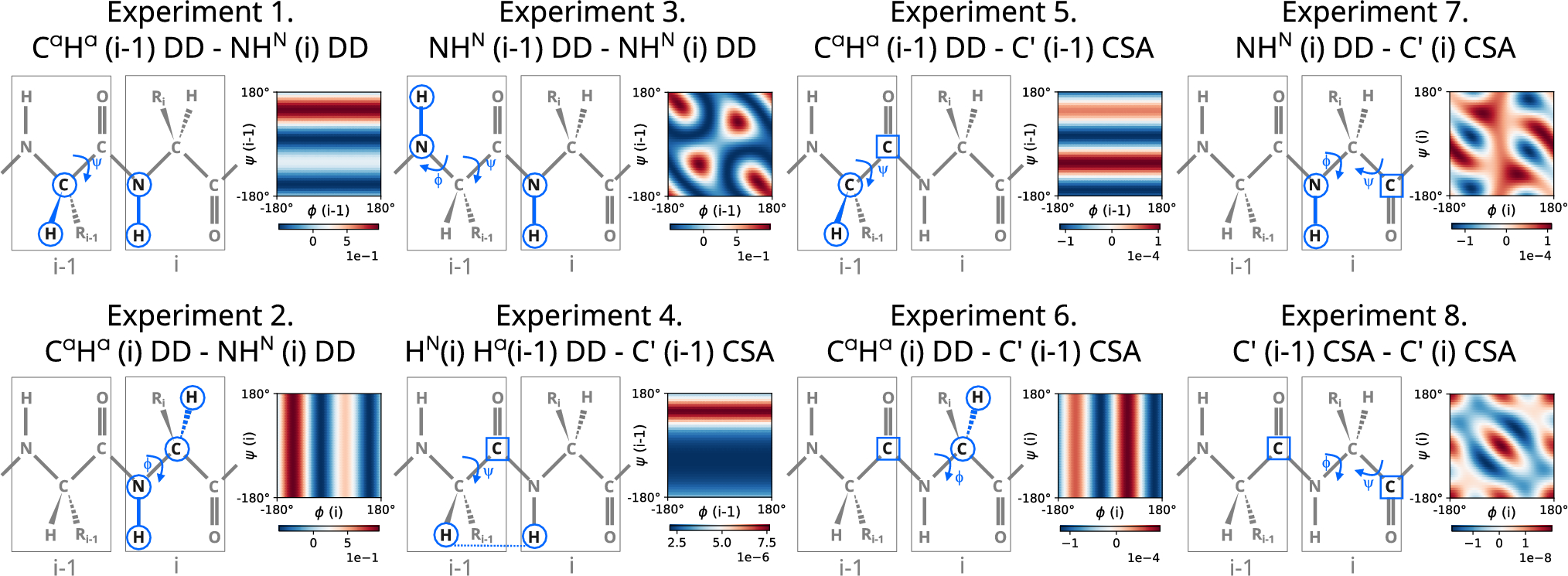
Cross-correlated relaxation (CCR) describes the interference between two simultaneously active relaxation mechanisms with equal tensor rank. For the most commonly considered mechanisms in solution-state NMR, dipolar (DP) and chemical shift anisotropy (CSA), these interference effects are encoded by time correlation functions (TCFs) of the form

$$\begin C_},}}(t) = \langle P_2(}(0) \cdot }(t)) \rangle \end$$

(1)

in isotropic solution. \(P_2(x) = 1.5x^2-0.5\) is the second order Legendre polynomial, \(}\) and \(}\) are motional vectors corresponding to dipolar unit vectors or principal components of CSA tensors, and angled brackets denote the ensemble average. For simplicity, we omit the contributions of time-dependent fluctuations of dipolar distances and/or CSA tensor geometries for now. These effects are addressed in more detail in the “Methods” section.

Identifying the dot product as the cosine of the projection angle \(\theta _},}}\), we see that the TCF encodes the average degree of correlation in \(P_2(\cos \theta _},}}\)) between \(}\) and \(}\) as a function of t. For the considered “remote” CCR interferences, which do not share any spin between the two relaxation mechanisms, the observable rate \(\Gamma\) is proportional to the spectral density at zero frequency, or, in case of a fully anisotropic CSA tensor, a linear combination of zero spectral densities. Considering the simpler case as an example for now, we obtain:

$$\begin \Gamma _},}} \propto J_},}}(0) = \int _0^\infty C_},}}(t) \,dt \end$$

(2)

Thus, the CCR rate encodes both structural and dynamical information about the relation between \(}\) and \(}\), albeit in rather convoluted fashion. Formally, one can separate the two components to obtain a more intuitive expression:

$$\begin J_},}}(0) = C_},}}(0) \int _0^\infty \frac},}}(t)}},}}(0)} \,dt = \langle P_2(}(0) \cdot }(0)) \rangle \tau _},}} \end$$

(3)

Dividing the TCF by its amplitude \(C_},}}(0)\), it is normalized, i.e. it starts off at 1. The integral of the normalized TCF is defined as the correlation time \(\tau _},}}\); it represents all relaxation mechanisms that affect \(C_},}}\) and is often called the "effective correlation time" in the context of NMR. The amplitude is the initial (“static”) population average at \(t = 0\). By adopting a model backbone geometry with \(\phi\) and \(\psi\) as the only conformational degrees of freedom, we can approximate \(C_},}}(0)\) as an average over an underlying dihedral angle distribution \(}_\):

$$\begin & \langle P_2(}(0) \cdot }(0)) \rangle = \langle P_2(\cos \theta _},}}(\phi ,\psi )) \rangle \nonumber \\ & \approx \sum _ p_ P_2(\cos \theta _},}}(\phi ,\psi )) \end$$

(4)

Anticipating the subsequent numerical implementation, we already denote the distribution \(}_\) as a finite probability vector; its entries \(p_\) act as the weights in a weighted sum defining the ensemble average. In the following, subscripts \(}\), \(}\) are dropped for convenience or replaced when indicating specific correlated components.

To make sense of CCR rates we must know either C(0) or \(\tau\). For folded proteins, both components can be reasonably approximated: \(}_\) could be known from a structural model; \(\tau\) mostly follows the rotational tumbling time of the protein. The case of a flexible backbone is more complex: C(0) results from an unknown and broadly populated \(}_\), while \(\tau\) does not follow a simple analytical model, encoding site-specific local motions, i.e. dynamics is heterogeneous along the protein backbone. In fact, the angular degrees of freedom governing the amplitude of the TCF might also affect its decay (Kämpf et al. 2018). Thus in disordered proteins, separation of C(0) and \(\tau\) is more involved than in structured proteins.

The investigated CCR rates \(\Gamma\) are defined by (linear combinations of) J(0), i.e. time integrals from 0 to \(\infty\) of TCFs with specific correlated components \(},}\), combined with the corresponding pre-factors (see Appendix). In principle, CCR rates are convoluted observables of a structural component \(A_\), representing the rates when C(0) is used instead of time integrals J(0), and a dynamical component \(\tau _\), described by the decay of the underlying TCFs, i.e. the time integrals of the normalized TCFs, see Eq. (3). Unfortunately, in an experimental context neither \(A_\) nor \(\tau _\) are directly accessible, but only their product \(\Gamma\). Therefore, in systems with heterogeneous dynamics, it is necessary to define an approximation for \(\tau _\) to be able to predict \(}_\) from a set of \(A_\) of different remote CCR rates \(\).

For a folded protein such as Ubiquitin, \(}_\) can be extracted with reasonable accuracy for a broad range of assumed \(\tau _\); all CCR rates were assumed to experience the same, slightly down-scaled tumbling time of the protein. While rates predicted from this simple model deviated considerably from experiment, \(}_\) could still be extracted with sufficient accuracy. Essentially, it was found that the main source of variation between rates lies in their amplitudes, not in their decay (Kauffmann et al. 2021).

In IDPs, correlation times are expected to be more heterogeneous, i.e. spin relaxation is more local in nature and does not follow the overall tumbling of the protein (Kämpf et al. 2018). Therefore, we need to identify how to best measure these local dynamics. For auto-correlated rates and other rates with known amplitude, the correlation time can be extracted directly from experiment. A straightforward and commonly measured option is the relaxation of the NH dipolar vector; its zero spectral density can be mapped through various experimental strategies (Kadeřávek et al. 2014) and provides a direct, residue-resolved measure of the local correlation time. Alternatively, we recently proposed a set of experiments to probe the correlation time related to the the \(C'C_\) bond (Loth et al. 2005; Kauffmann et al. 2021). Presuming for now that such estimates are indeed capable of approximating the correlation times of nearby remote CCR interactions, we can construct a suitable model to extract \(}_\).

First, we will formalize the general problem in the language of Bayesian statistics. Given a set of CCR rates \(\Gamma _1,\ldots ,\Gamma _j\), denoted as a vector \(\varvec\), we want to infer the underlying distribution \(}_\). Assuming for now that the correlation times are known, the observed CCR rates are a function of \(}_\) alone. We then write this problem as a conditional probability, i.e. we assign any realization of \(}_\) a probability P given the data \(\varvec\). Rearranging this expression,

$$\begin P(}_\vert \varvec)&= \dfrac}_\cap \varvec)})} = \dfrac}_\cap \varvec)}}_)}P(}_)})} \nonumber \\ &= \dfrac\vert }_)P(}_)})} \end$$

(5)

yields Bayes’ theorem. It provides a way to calculate the quantity of interest, the posterior probability \(P(}_\vert \varvec)\), by evaluating the likelihood \(P(\varvec\vert }_)\) and the prior \(P(}_)\). Since we are only interested in comparing the relative probabilities of different \(}_\), i.e. we take the observed data \(\varvec\) as given, we can omit the evidence \(P(\varvec)\). Bayes’ theorem then reads: posterior \(\propto\) likelihood \(\times\) prior. Evidently, Bayesian inference does not single out one ’solution’, rather it produces a probability distribution over different realizations of \(}_\); a result that is very general but also quite cumbersome. Often, one is interested in obtaining simpler and more convenient point estimates for \(P(}_\vert \varvec)\).

For the likelihood, we will adhere to the commonly made assumption of uncorrelated Gaussian errors:

$$\begin P(\varvec\vert }_) \propto \exp \bigg (-\sum _^m \frac}_}}) -\Gamma _j)^2}\bigg ) \end$$

(6)

The smaller (the sum of) the \(\chi ^2\) between the functions \(\Gamma _j (}_}})\) and the observed rates \(\Gamma _j\) are, the higher is the probability of the underlying \(}_\). The variances \(\sigma _j^2\) quantify the experimental uncertainty (Kauffmann et al. 2021) associated with each rate (and thus are set to 1 for the purposes of this work).

The prior \(P(}_)\) requires more consideration. Encoding our intuition and knowledge about the problem, it contains the solutions we allow for a priori. For example, in our first implementation(Kloiber et al. 2002), we presumed a rigid fold, i.e. only point-like distributions \(}_\) were considered, effectively negating all ensemble-averaging effects. Preferring no one (\(\phi\), \(\psi\))-pair over another, i.e. assuming a uniform prior, the posterior could then be visualized and evaluated simply as a function of \(\phi\) and \(\psi\).

To model a more flexible backbone, the prior \(P(}_)\) must allow for more broadly populated distributions. Not only do we need to account for ensemble averaging effects explicitly, we also must anticipate the increased ambiguity they might introduce: A more general prior might contain many different \(}_\) with similar \(\chi ^2\); the likelihood flattens, so to speak. With the intention to derive a simple point estimate for \(}_\), the prior must be shaped accordingly.

A common strategy is to employ an entropy prior, which can be derived from first principles (Skilling 1989; Gull 1989) or introduced more ad hoc (Hummer and Köfinger 2015):

$$\begin P(}_) \propto \exp \bigg (-T\sum _ p_ \log \frac}}\bigg ) \end$$

(7)

The closer \(}_\) is to \(}_\) in terms of its relative entropy or Kullback–Leibler divergence \(D_\), the higher is its probability. Similarly to the variances \(\sigma _j^2\), the scaling factor or “temperature” T quantifies the confidence in \(}_\), i.e. the prior expectation for \(}_\) before observing any data.

The practical reason for employing this prior lies in the convexity of \(D_\). A distribution over possible distributions is quite cumbersome to evaluate. To simplify further, we pick the maximum of \(P(}_\vert \varvec)\), i.e. the most likely realization, as a representative point approximation in a Maximum A Posteriori (MAP) estimate. Noting that \(\max (\exp ) = \max (\log (\exp )) = \min (-\log (\exp ))\), we obtain a familiar optimization problem:

$$\begin \min _}_}\; D_(}_\Vert }_) \cdot T + \sum _^m \frac}_}}) -\Gamma _j)^2} \end$$

(8)

We obtain a simple regularized \(\chi ^2\)-fit using an entropy penalty. Not by coincidence, this expression corresponds to the well-known Maximum Entropy (MaxEnt) formalism first proposed by Gull and Daniell (1978). The above generalization in Bayesian terms was first derived by Skilling (1989) and Gull (1989) and recently rediscovered by Hummer and Köfinger in the context of structural biology(Hummer and Köfinger 2015; Köfinger et al. 2019). Practical differences generally revolve around the treatment of the free parameter T. Here, T will simply be optimized to achieve a sensible balance between \(\chi ^2\) and \(D_\) using an L-curve heuristic (Miller 1970; Hansen 1992). Again, instead of a fully Bayesian treatment (Bryan 1990), we resort to simpler point estimates.

The central question of this study is whether the proposed approach can yield a good approximation for \(}_\). Since this is expected to partially depend on the characteristics of the investigated system, we consider both folded proteins and IDPs.

For folded proteins like Ubiquitin, experimentally derived ensemble representations are available (Lange et al. 2008); assessing the validity of the proposed approach is thus straightforward(Kauffmann et al. 2021). For IDPs, one lacks experimental “ground truth” and must resort to an asserted representation of the ensemble and its dynamics. Arguably, molecular dynamics (MD) simulations provide the best structural and dynamical models for IDPs available to date (Rauscher et al. 2015; Robustelli et al. 2018; Piana et al. 2020). For the intended purpose of validation, MD simulations can serve as a self-contained framework that extends beyond the limits of analytical models.

In a first step, CCR rates are calculated from simulated trajectories and, in analogy to experimental procedure, subsequently processed to yield \(}_\). Next, these results are compared to a reference distribution \(}_\) as observed directly in the underlying trajectories, assessing the validity and limitations of the proposed protocol (Kämpf et al. 2018; Bremi and Brüschweiler 1997; Case 2002; Prompers and Brüschweiler 2002).

Force fields for biomolecular and particularly IDP simulations have drastically improved in recent years. Here, we employ an advanced model called des-amber (Robustelli et al. 2018) that was developed to cover a broad range of systems. More specifically, it is suitable for both ordered and disordered proteins and was further refined with an emphasis on non-bonded potentials. While the motivation for the development of the last iteration of this force field family was a better description of intermolecular interactions between biological macromolecules, we believe that it can have additional merits compared to previous force fields even in the case of a single-chain disordered system, considering the frequent occurrence of transient interactions between remote residues.

It is worth noting that quantitative agreements with experiments are by no means a strict requirement for the intended purpose of this study. As long as the characteristics of the simulation can be considered a realistic representation of the generic structural dynamics of proteins/IDPs, the general workflow of predicting \(}_\) from CCR rates can be validated in a fully self-consistent manner, namely by comparison to the reference distribution \(}_\) calculated from the same underlying simulation data.