1 Introduction

Hypertension (HTN) has been well recognized as a major risk factor for morbi-mortality of cardiovascular diseases (1). Since 1990 the number of people with hypertension worldwide has doubled (2). Two decades later it has been reported that one in three people has hypertension and around 40% of adults over 25 years of age are diagnosed with hypertension worldwide (3). Hypertension has been associated to more than 10 million deaths per year, 9 million deaths from stroke, ischaemic heart disease, other vascular diseases, and renal disease, and for more than 23 million disability-adjusted life years lost worldwide (4, 5). The most recent prevalence of hypertension has been estimated around 30% to 45% among the adult population across the world and remained almost the same between men and women (6), varying by age, regions and national income (4, 7, 8).

The presence of hypertension is rising globally owing to ageing of the population and increases in exposure to lifestyle risk factors including lack of physical activity, anxiety and sleep quality (9, 10). Common determinants such as nutritional, environmental and behavioural factors of hypertension vs. normotensive at the individual level are well-established (11–13). Substance abuse such as excessive caffeine consumption through the intake of energy drinks related to other factors such as stress, excessive workload and insomnia are also proposed as emerging factors related to early-onset hypertension (14–16). On the other hand, declining mobility (17), as well as, occupational or domestic physical activity (12, 18) and transportation physical activity (19), have also been explored as factors related to develop hypertension in relatively-young adult people.

In México, the prevalence of hypertension in adults older than 20 years of age was reported to be 29.4% (27.7% in women and 31.3% in men) according to the 2022 National Health and Nutrition Survey (Ensanut 2022) (20). Of the total Mexican population with hypertension, around 47% are unaware of their diagnosis (21). However, even in the most populous city nationwide, with just over nine million inhabitants, there is still a lack of specific information regarding common and emergent hypertension risk factors, especially in relatively young adults and without any other apparent disease.

In response to the escalating prevalence of hypertension, this study has taken a data-driven approach by implementing machine learning models, including the extreme gradient boosting (XGBoost), Support Vector Machines (SVM), and Shapley Additive exPlanations (SHAP), to explore the factors associated with new-onset hypertension in initially healthy adults participating in the Tlalpan 2020 cohort study. Recent studies underscore the potential of machine learning in revealing intricate relationships within health data, particularly for populations at heightened risk of undiagnosed hypertension (22).

The implementation of models such as XGBoost in studies on hypertension factors has been a growing trend due to the algorithm’s capability to extract meaningful features and patterns. In their study, Chang et al. (23) utilized the GSFTS-FS method for feature selection and XGBoost to predict outcomes in the context of hypertension. The proposed model outperformed others by 10%, achieving high accuracy (0.95) and AUC (0.96) using cross-validation method. Additionally, Peng et al. (24) developed a hybrid model for hypertension detection, combining LASSO regression for feature selection and XGBoost for prediction. Achieved 77.2% of accuracy and 84.6% of AUC.

Moreover, techniques like SHAP have proven pivotal in hypertension prediction within machine learning (25). Miranda et al. (26) utilized SHAP to identify specific contributions of features, enhancing the performance of the Random Forest model. This improvement enabled the model to distinguish between hypertensive and normotensive patients with an accuracy of 84.2%, specificity of 78.0%, and sensitivity of 84.0%. In another study (27), researchers tackled the heightened risk of COVID-19 mortality among hypertensive patients. They employed a feature filtering algorithm for selecting relevant features and utilized SVM to predict food-derived antihypertensive peptides. The SVM model demonstrated accuracies of 86.17% and 85.61%, suggesting a promising approach for the management of hypertension.

The primary goal of this study is to explore emerging risk factors for early-onset hypertension using a data-driven approach and machine learning models within a well-established cohort in México City. Recognizing hypertension as a significant public health concern with complex and variable determinants, the research aims to identify factors beyond those currently recognized, which account for only a fraction of the observed prevalence. By analyzing data from initially healthy adults aged 18 to 50 years over a five-year follow-up period, this study employs machine learning models such as Extreme Gradient Boosting, Support Vector Machines, and Random Forest alongside Shapley values to assess the influence, direction, and contribution of a range of lifestyle, anthropometric, clinical, and biochemical variables to extend the current knowledge of hypertension’s determinants, bothbin the general case as well as in a sex-stratified analysis.

2 Methods 2.1 Study design and participants

The Tlalpan 2020 cohort is an observational, longitudinal, prospective study that was conducted at the Instituto Nacional de Cardiología Ignacio Chávez (INCICH), one of the National Institutes of Health and a public flagship hospital institution for the treatment of cardiovascular diseases in México. The main objective of the Tlalpan 2020 study is to evaluate the effect of traditional and non-traditional risk factors on the incidence of HTN in a cohort of México City (28).

The recruitment period was from September 2014 to June 2019. The inclusion criteria were: men and women (not pregnant or lactating) between twenty and fifty years old who live in México City; without history of cardiovascular diseases, not diagnosed with cancer with an effect on survival or with cognitive and mental disabilities; without chronic infections, inflammatory and/or immune disorders; and who agree to participate in the study. The exclusion criteria included participants identified with hypertension or diabetes during the baseline survey, as well as those who failed to provide complete information. The elimination criteria during follow up were: people who did not wish to continue participating or it was not possible to re-contact; those who changed their address outside of México City; as well as those who have developed cardiovascular disease or died.

2.2 Institutional review board statement

The Tlalpan 2020 study was approved by the Institutional Bioethics Committee of INCICH under number 13-802. This study was conducted according to the guidelines laid down in the Declaration of Helsinki (29).

2.3 Data elements and measurement scales

A set of standardized questionnaires was applied, on a face-to-face interview, to collect information on demographic characteristics: Marital status (single, married and other), highest educational level concluded (elementary school, junior high school, college and postgraduate), occupational class (student, business executive, housekeeper, professional, manually qualifies, manually unqualified, other and unemployed). Also, data of lifestyle habits and family medical history were recorded. Macro and micronutrients intake were calculated using the Evaluation of Nutritional Habits and Nutrient Consumption System obtained by a semi-quantitative food frequency questionnaire (SFFQ) with 140-item about dietary sources of energy, protein, carbohydrate, dietary fiber, total fat, saturated fatty acids (SFAs), monounsaturated fatty acids (MUFAs) and polyunsaturated fatty acids (PUFAs) (30). Physical activity was measured by the long version of International Physical Activity Questionnaire, IPAQ: categorized into low, moderate, or high physical activity levels. Psychological stress level was determined by the State-Trait Anxiety Inventory, STAI Spanish version (31), and sleep disorders by means of the Spanish-language Medical Outcomes Study-Sleep scale (MOS) of twelve items (32).

Anthropometric measurements (weight, height and waist circumference) were recorded during physical examination. Body weight and height were measured using a calibrated stadiometer SECA 220 and a mechanical column scale (SECA 700) with a capacity of 220 kg and precision of 0.05 kg with participants wearing light clothing and no shoes. Body mass index (BMI) was calculated as usual by taking the participant’s weight in kilograms divided by height in meters squared. Waist circumference (Waist-size) was measured at the level of 1 cm above the umbilicus. Smoking status was defined as: (1) Currently smoking, ever having smoked at least 100 cigarettes in a lifetime (Hundred-cigarettes), (2) Formerly smoked, previously smoked, had a lifetime consumption of over 100 cigarettes or currently abstains from smoking and (3) Passive smoker. Alcohol consumption was defined as the consumption of any type of alcoholic beverage at least 12 times in the last twelve months (28).

Laboratory measurements were also obtained and the biochemical data were validated in automatic analyzers at the Central Laboratory of INCICH using standardized procedures. Blood samples were obtained after an overnight fast of twelve hours (12 h). Samples were measured by Automated Photometry, Spectrophotometry, Potentiometry and Chemiluminescence and were run on the AU 680 Beckman Coulter (2012). Coulter LH Series Pak Reagent Kit. The values references of the laboratory parameters were: fasting plasma glucose (70–105 mg/dl), triglycerides (40–200 mg/dl), low-density lipoprotein cholesterol (LDL-cholesterol) (80–130 mg/dl), high-density lipoprotein cholesterol (HDL-cholesterol) (women: >50 mg/dl and men: >40 mg/dl), total cholesterol (140–200 mg/dl), uric acid (women: 3.80–6.20 mg/dl and men: 4.80–8.00 mg/dl), serum creatinine (women: 0.60–1.00 mg/dl and men: 0.70–1.30 mg/dl), Atherogenic index (LDL-cholesterol/HDL-cholesterol, elevated defined as a value >4) and serum sodium (136.00–145.00 mmol/l). Also, complete blood count parameters (counts of white blood cells, red blood cells and platelets, the mean corpuscular hemoglobin (MCH), the hematocrit and the mean platelet volume (MPV)) were examined (28)

A urine sample from a twenty-four hour (24 h) period was also obtained. For a proper urine collection, the participant was given precise and clear indications (discard the first urine in the morning and collect all urine for a period of 24 h, including the first urine of the following morning, which will be the day of the appointment). Urinary sodium and potassium were determined by the ion selective electrode method, and urinary creatinine was determined by Jaffe’s colorimetric assay using an automated analyser. The urine sample will be considered to be complete when urinary creatinine levels are within the standard creatinine excretion rate. The reference values of urinary variables are following: for creatinine in women between 740–1570 mg/24 h and for men between 1040–2350 mg/24 h, for sodium between 40.00–220.00 mmol/24 h and for potassium excretion between 25.00–125.00 mmol/24 h. Sodium and potassium excretion was reported in mmol/24 h (or equivalently mEq/24 h) (28).

2.4 Hypertension definition

The primary outcome of the Tlalpan 2020 study was the development of elevated blood pressure (BP) during 6,000 person-years of follow-up. The development of hypertension was defined as a previously normotensive participant whose systolic blood pressure (SBP) was ≥140 mm Hg and/or their diastolic blood pressure (DBP) was ≥90 mm Hg after at least three repeated examinations (28, 33).

2.5 Office blood pressure assessment

Participants were advised to have an empty bladder, not to exercise and not to smoke, drink coffee or tea, for at least 30 min before office BP measurements. Participants were seated in a quiet room (neither participant nor staff talked before, during and between measurements) with comfortable temperature for at least 5 min before the first evaluation, arm resting on table with the mid-arm at heart level; back supported on a chair; legs uncrossed and feet flat on the floor. Blood pressure was measured in the left arm three times with a three min interval between each measurement. If one of the three measurements is quite different, a four measure is taken. The value recorded is the average of the three closer measurements.

During the follow-up, all participants were contacted by telephone every 12 months to verify whether they have been diagnosed with hypertension. The main questions asked to them –based on previous studies– (34–37) were: Has a doctor or other health provider ever told you that you have hypertension? Participants who reported a hypertension diagnosis were then asked about current use of medication to lower BP: Are you currently taking any medicines, tablets, or pills for hypertension? and In the last few weeks, have you taken any drug (medication) that could have affected your blood pressure? In affirmative cases, all the details related to symptoms, diagnosis and pharmacological treatments are requested and documented in the medical file. We define an onset case of hypertension when those participants attend the INCICH to confirm the diagnosis by our team of clinical collaborators and to complete the “end of the study follow-up” visit format. Therefore, the date of disease onset is considered as the date of confirmation of the diagnosis or the date of anti-hypertensive treatment start. For those diagnosed with hypertension during one of the stages of follow-up visits, in every case, the date of disease onset is recorded as the date of the visit.

2.6 Selection of hypertensive and normotensive individuals

Of the 3,000 participants who were free of hypertension at the baseline examination, 2,500 took part in monitoring until the year 2023 at five years on average from the start of recruitment. Among them, 150 developed hypertension during follow-up and 2,350 participants remained without hypertension. For each hypertensive case, four counterparts without hypertension remained were selected throughout the same time interval and matched for gender and age (±2 years); 750 participants (150 hypertensive and 600 normotensive individuals) were eligible for final analysis.

2.7 Machine learning methods

In this study, we implemented a comprehensive approach that combines various strategies to enhance the understanding of the determining risk factors related with the development of hypertension. We applied data balancing techniques and attribute selection, supported by machine learning algorithms, to identify the most relevant features (See Figure 1).

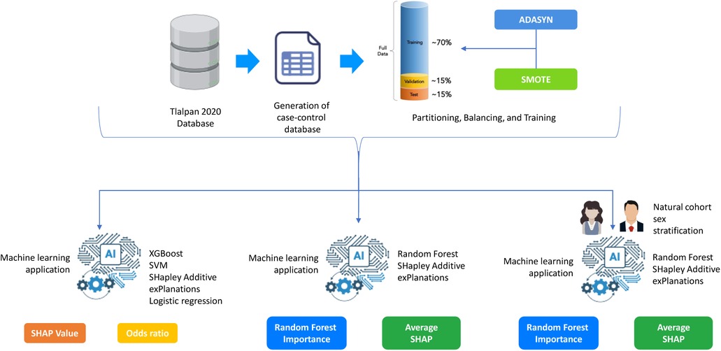
Figure 1. General Methodology for Hypertension Risk Prediction Using Machine Learning.

2.7.1 Data balancing techniques

To counteract class distribution imbalance, mitigate associated adverse impacts, and address dimensional complexity, we implemented the techniques of SMOTE (Synthetic Minority Over-sampling Technique) and ADASYN (Adaptive Synthetic Sampling). SMOTE generates synthetic instances of the minority class by interpolating between existing samples, providing additional variability, and strengthening the representation of the less frequent class (38). Conversely, ADASYN further advances the concept introduced by SMOTE by adjusting the density of synthetic samples in proportion to the local distribution of the minority class (39). Both techniques have been widely employed to balance datasets and enhance the performance of machine learning models applied in the health sector (40, 41).

2.7.2 XGBoost

After achieving a balance in the data through data balancing techniques, we applied the XGBoost algorithm not only as a machine learning model but also as a feature selection tool. XGBoost belongs to the ensemble model category, utilizing decision trees as base components. Mathematically, XGBoost’s training involves optimizing a cost function, quantifying the discrepancy between model predictions and actual values (42).

2.7.3 Support vector machines (SVM)

Support Vector Machine (43) operates by finding the optimal hyperplane that maximizes the separation between classes in a multidimensional space. It transforms the data into a higher-dimensional feature space, seeking a hyperplane that maximizes the margin between classes. In this study, SVM was utilized with a radial kernel. The choice of the radial kernel was based on observed results, demonstrating improved performance according to the balanced accuracy metric.

2.7.4 SHapley Additive exPlanations (SHAP)

SHapley Additive exPlanations is a concept from game theory (44) that has been successfully applied to assess the contribution of each feature to a model’s predictions. In this study, Shapley Values were employed to identify features related to hypertension. The subset of features obtained through Shapley Values was subsequently evaluated using a support vector machine with a radial kernel (see Equation 1). The Shapley Values are defined by:

ϕi(v)=∑S⊆N∖|S|!(|N|−|S|−1)!|N|!(v(S∪)−v(S))(1)

Where:ϕi(v) is the Shapley Value of player. N is the set of players. v is the characteristic function assigning a value to each coalition of players. S is a coalition of players that does not contain player i. |S| is the number of players in coalition S. |N| is the total number of players.

2.7.5 Random forest

Random Forest, developed by Leo Breiman in 2001, is a machine learning algorithm that combines multiple decision trees to improve accuracy and reduce overfitting. By creating a forest of decision trees, each trained on a random subset of the data and features, the model makes a final prediction based on majority voting. In Python, key parameters such as n_estimators (the number of trees), max_depth (the maximum depth of each tree), min_samples_split (the minimum number of samples required to split a node), and max_features (the maximum number of features considered at each split) allow fine-tuning of the model to optimize performance and reduce overfitting. A key feature of Random Forest is its ability to calculate Variable Importance Percent, which quantifies each feature’s contribution by measuring the reduction in impurity across all trees. Higher importance scores indicate a stronger influence on predictions, highlighting the most impactful variables.

2.7.6 Performance evaluation metrics

Sensitivity (SEMS) measures the model’s ability to correctly identify positive instances, while specificity (SPC) assesses its ability to accurately classify negative instances. Balanced accuracy (B.ACC) considers both proportions, providing a comprehensive measure of the model’s overall performance. In health contexts, where the accurate identification of both positive and negative cases is critical, these metrics provide a comprehensive view of the model’s performance (see Equations 2–4). The equations are defined by: ?>

SEMS=TPTP+FN(2)

SPC=TNFP+TN(3)

B.ACC=(12)(TPP+TNN)(4)

In this context, P represents positive instances, N represents negative instances, and TP, FN, TN, and FP denote true positives, false negatives, true negatives, and false positives, respectively.

The Jupyter Notebook environment (version 6.4.12) was employed for developing and evaluating machine learning models, as well as designing network calculators, using Python (version 3.9.13). For handling class imbalance in the dataset, both ADASYN and SMOTE were implemented. Additionally, SHAP was utilized for feature importance and selection. The computer equipment utilized consisted of a Dell workstation, featuring an Intel(R) Xeon(R) Core processor, 32 GB of RAM, and a processor speed of 3.50 GHz, with Windows operating as the system.

2.8 Statistical analysis

The baseline characteristics of hypertensive and normotensive individuals were compared using Pearson’s chi-squared test for categorical variables and Wilcoxon test for continuous variables. The distribution of numerical data was assessed using the Shapiro-Francia tests. Analyses were performed using [R] version 4.0.2 (45).

2.8.1 Experimental design configuration

Firstly, data balancing techniques were implemented with the aim of ensuring optimal performance of the models and feature selection. This phase addressed potential imbalances in the class distribution, ensuring that the models could learn equitably from all instances and, consequently, enhance their overall performance. Subsequently, a dataset partition was conducted, allocating 70% for training and 30% for testing. Additionally, a 10-fold cross-validation strategy was configured. This choice is grounded in the need to obtain more reliable estimations of the model’s performance by training and evaluating it repeatedly on different subsets of data.

For parameter selection after configuring the 10-fold cross-validation, a grid method was employed. For XGBoost, the following parameter grid in was varied: max_depth, learning_rate, and n_estimators. Similarly, for SVM with kernel RBF, the parameter grid included C and gamma. This additional step aims to find the optimal parameter combination that maximizes the predictive performance of the models. Finally, the selected subsets of features and parameters were put to the test in the models. A similar experimental design was implemented for the sex-stratified analysis.

3 Results 3.1 General characteristics of the participants

The primary outcome was the development of hypertension during 6,000 person-years of follow-up. Of the 150 participants who developed hypertension 61.33% was women of median age 50 (47–55 IQR) and 38.67% was men of median age 48 (42–53 IQR) (see Supplementary Table S1). Six hundred normotensive participants were selected to match them by sex and age. Once the data of the sociodemographic, anthropometric, family pathological history, lifestyles and clinical evaluations were obtained and compared –between men and women with and without hypertension– some features stand out: The majority of women with hypertension were classified in the low SDI group (24%), while the highest proportion of men with hypertension was found in the high SDI group (18%). Despite these differences, both groups had a higher prevalence of individuals with advanced education and employment in skilled or professional occupations (see Supplementary Table S2).

A higher percentage of smokers (active or passive) was reported in cases of hypertension, 32% vs. 29.88% in smoking women and 32% vs. 29.38% in smoking men (see Supplementary Table S1). Most of the participants –hypertensive and normotensive –apparently in good health were overweight, BMI of women was 28.46 (25.97–34.22 IQR) vs. 26.59 (23.80–29.72 IQR), and BMI of men was 28.46 (26.83–31.16 IQR) vs. 26.91 (24.21–29.92 IQR), see Supplementary Table S1.

Women and men with new-onset hypertension reported a higher percentage of risk factors than normotension such as: father with obesity, 12% and 8.67%; smoking mother, 6.67% and 8%; mother with diabetes, 18.67% and 8.67%; father with diabetes, 21.33% and 8%; mother with hypertension, 28% and 14.67%; father with hypertension, 19.33% and 12.67% –see Supplementary Table S3. A greater number of minutes spent sitting at day was reported among cases that developed hypertension vs. those who remained normotensive: 300 min (180–420 IQR) vs. 240 min (120–360 IQR) in women and 300 min (180–480 IQR) vs. 240 min (180–480 IQR) in men (see Supplementary Table S4).

Clinical parameters with a statistically significant difference between hypertensive and normotensive were: HDL-cholesterol mg/dl 47 vs. 49.35 (pvalue=0.0359) in women and 38.85 vs. 41.50 (pvalue=0.0118) in men; and the triglycerides only between men 194.85 vs. 153.90 (pvalue=0.0077) (see Supplementary Table S4). The Supplementary Materials provide additional descriptive data on the cohort, including details on sociodemographic factors, anthropometric measurements, family history of disease, sleep characteristics, physical activity, psychological stress, and the consumption of tobacco, alcohol, or energy drinks. They also include information on basic clinical parameters, food and nutrient consumption reports and complete blood count results.

3.2 Machine learning results

To deepen the evaluation of the model’s performance in predicting hypertension, three analyses were conducted to assess the influence, direction, and relative importance of individual features that improve the model’s predictive accuracy from the natural cohort (prior to matching). Subsequently, a sex-stratified analysis was performed to identify potential gender-specific risk factors. To illustrate the methodological workflow implemented in this study, Figure 1 provides an overview of the steps taken to analyze hypertension risk factors. The process begins with the Tlalpan 2020 Database, a comprehensive cohort dataset. A case-control dataset was generated to identify individuals with hypertension (cases) and matched controls. The data was then split into training (70%), validation (15%), and test (15%) sets. To address class imbalance, ADASYN and SMOTE were applied, ensuring balanced data for model training and more accurate feature importance assessment. These preprocessing steps established a solid foundation for predictive modeling and the identification of key hypertension risk factors.

The first analysis identifies the most important features based on their Shapley values, applying XGBoost and SVM algorithms along with resampling techniques such as ADASYN and SMOTE to balance the dataset. This step provides an initial understanding of the variables that hold the greatest influence in predicting hypertension, as determined by their Shapley contribution scores.

In the second analysis, Random Forest was employed to further validate the key features, using its Variable Importance Percent metric to highlight the most influential variables. Additionally, Shapley values were applied once more to these Random Forest results, allowing for a more detailed examination of each feature’s direction and level of contribution to hypertension risk. This combination of Random Forest importance scores and Shapley values enables a comprehensive view of whether each variable positively or negatively impacts hypertension prediction and to what extent.

Lastly, a gender-specific analysis was conducted by applying Random Forest separately for men and women to capture potential differences in feature importance by sex. Using Shapley values again in this gender-stratified analysis, along with ADASYN and SMOTE balancing techniques, this final evaluation reveals how each variable uniquely contributes to hypertension risk for men and women, adding another layer of interpretability to the model.

3.2.1 Feature importance analysis using extreme gradient boosting and support vector machines

In this section, we present the results of the most relevant variables identified using XGBoost and SVM, analyzed with SHAP values, in conjunction with ADASYN and SMOTE balancing techniques. The results include each variable’s average SHAP value, odds ratio, direction of influence (positive or negative), and an interpretation of the impact on hypertension risk.

The SHAP value plots (Figures 2, 3, 4, 5) visually represent the impact of each feature on the model’s predictions, where each point corresponds to an individual feature’s contribution. SHAP values along the x-axis indicate both the direction and magnitude of this influence: points extending further to the right suggest an increase in the model’s prediction, while those on the left indicate a decrease. High feature values are depicted in red, and their distance from the center (left or right) highlights the most influential features. Figure 2 shows the SHAP values for features balanced with ADASYN using XGBoost, while Figure 3 presents the features balanced with SMOTE in XGBoost. Figure 4 highlights the features identified by SVM with ADASYN, and Figure 5 displays those obtained by SVM with SMOTE.

Figure 2. Variable Significance with XGBoost, SHAP and ADASYN. Lack-air, Waking up feeling short of breath and/or headache; Sitting-mins-day, Minutes sitting per day; Waist-size, Waist circumference; BMI, Body mass index; MPV, Mean platelet volume; Sleep-adequacy, Adequate sleep report; Trait-anxiety, Anxiety as a trait; State-anxiety, Anxiety as a state; SS-Headache, Hours-fall-asleep and wake up with a headache; Low-physical-act, Low physical activity; Hours-fall-asleep, Hours to fall asleep; Take-naps, Take-naps of more than five minutes a day; SDI-Level, Social Development Index.

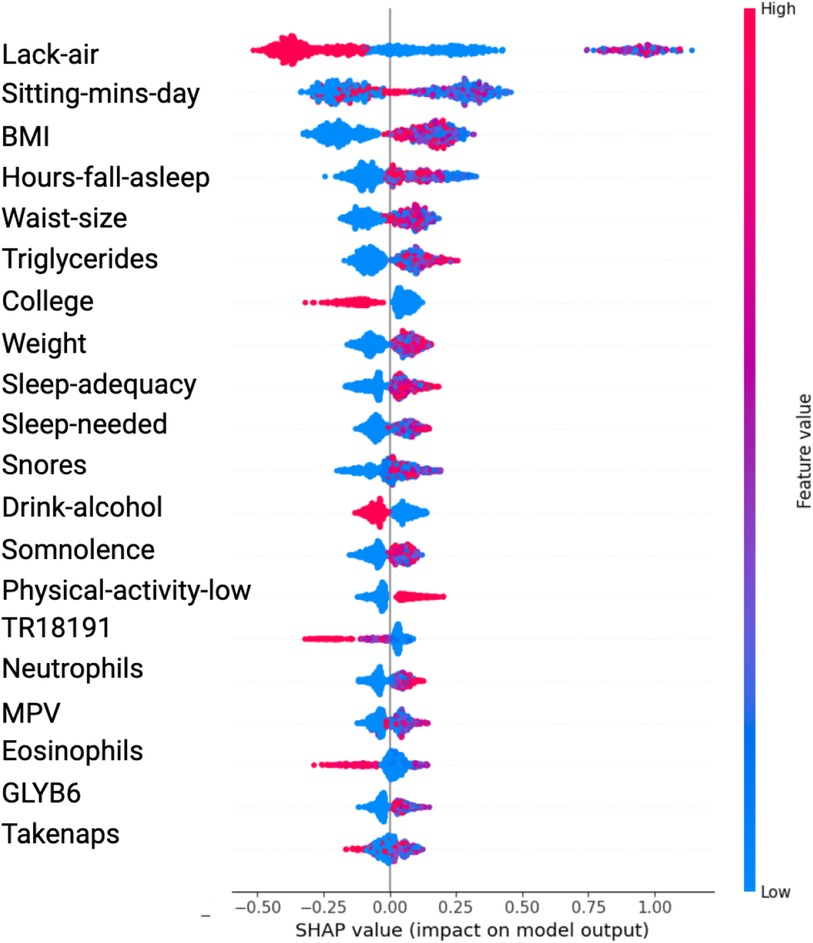
Figure 3. Variable Significance with XGBoost, SHAP and SMOTE Lack-air, Waking up feeling short of breath and/or headache; Sitting-mins-day, Minutes sitting per day; BMI, Body mass index; Hours-fall-asleep, Hours to fall asleep; Waist-size, Waist circumference; Sleep-adequacy, Adequate sleep report; Sleep-needed, Not getting enough sleep to feel rested when wake up in the morning; TR18191, Trans 18:1 fatty acid; MPV, Mean platelet volume; Take-naps, Take-naps of more than five minutes a day.

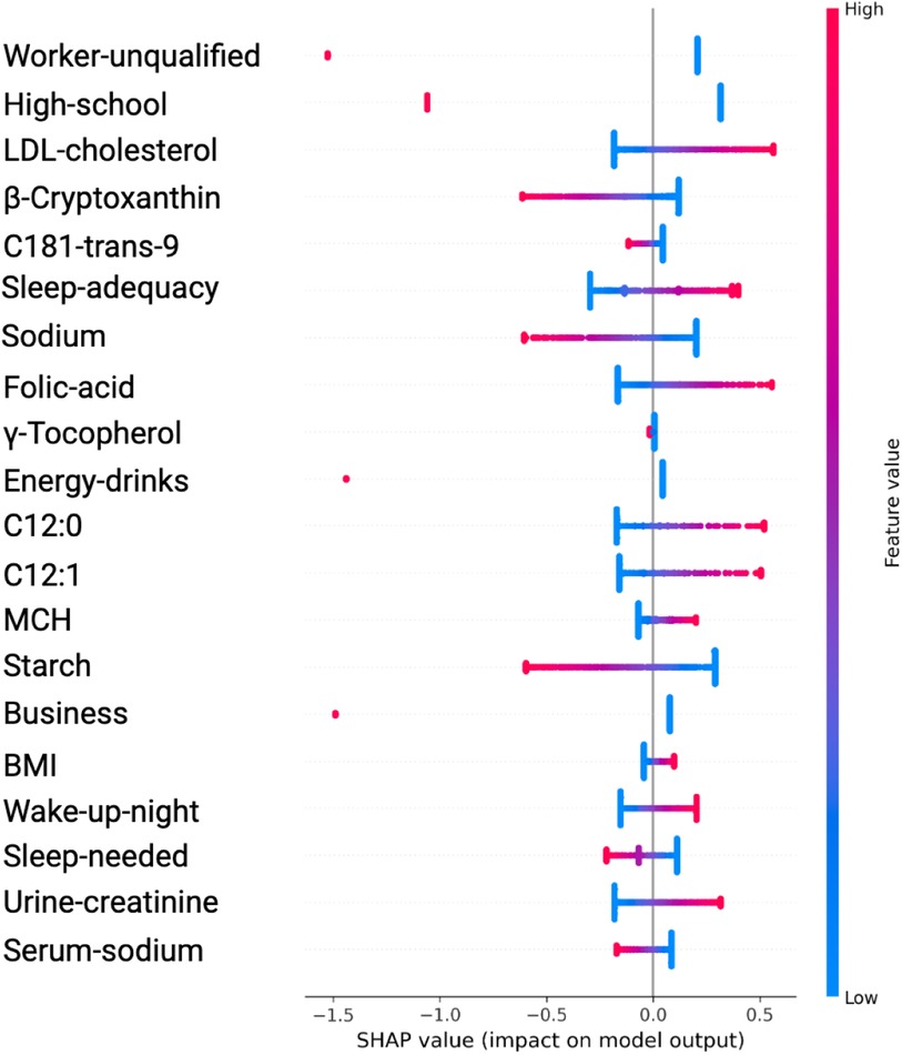
Figure 4. Variable Significance with SVM, SHAP and ADASYN. C181-trans-9, unsaturated trans fatty acid; MCH, mean corpuscular hemoglobin; C12:0 and C12, saturated fatty acids; Sleep-adequacy, Adequate sleep report; Sleep-needed, Not getting enough sleep to feel rested when wake up in the morning; β-Cryptoxanthin, carotenoids; γ-Tocopherol, tocopherols; Wake-up-night, Wakes up while sleeping and has difficulty going back to sleep.

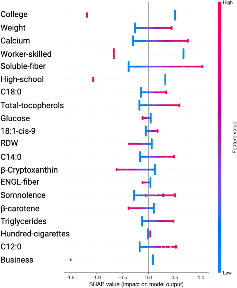
Figure 5. Variable Significance with SVM, SHAP and SMOTE. C18:0, C12:0, C14:0, specific saturated trans fatty acid; 18:1-cis-9, monounsaturated fatty acids omega-9; ENGL-fiber, dietary fiber; Hundred-cigarettes, consumption of more than 100 cigarettes; RDW, Red Blood Cell Distribution Widht.

Table 1 presents the significant variables identified through XGBoost and ADASYN, showing the average SHAP value and the odds ratio for each feature. The average SHAP value reflects the mean impact of each feature on the model’s predictions, while the odds ratio provides a quantitative measure of both the direction and strength of its influence. According to this table, the variables such as Lack-air (waking up feeling short of breath or with a headache), BMI and Waist-size, have a high SHAP value but an odds ratio of 0.1795, 0.5708 and 0.8577 respectively, indicating a reduction in hypertension risk for individuals with this feature. In contrast, Sitting-mins-day (minutes sitting per day) and Weight as well as Low-physical-activity and Hours-fall-asleep also have a high SHAP value but an odds ratio above 1, suggesting that sedentary behavior and obesity increases the risk of hypertension. Also, the Table 1 indicate that anxiety levels, whether as a personality trait (Trait-anxiety), has a positive influence on hypertension risk, with odds ratio of 2.5114. This suggests that persistent anxiety levels may be key factor in hypertension development.

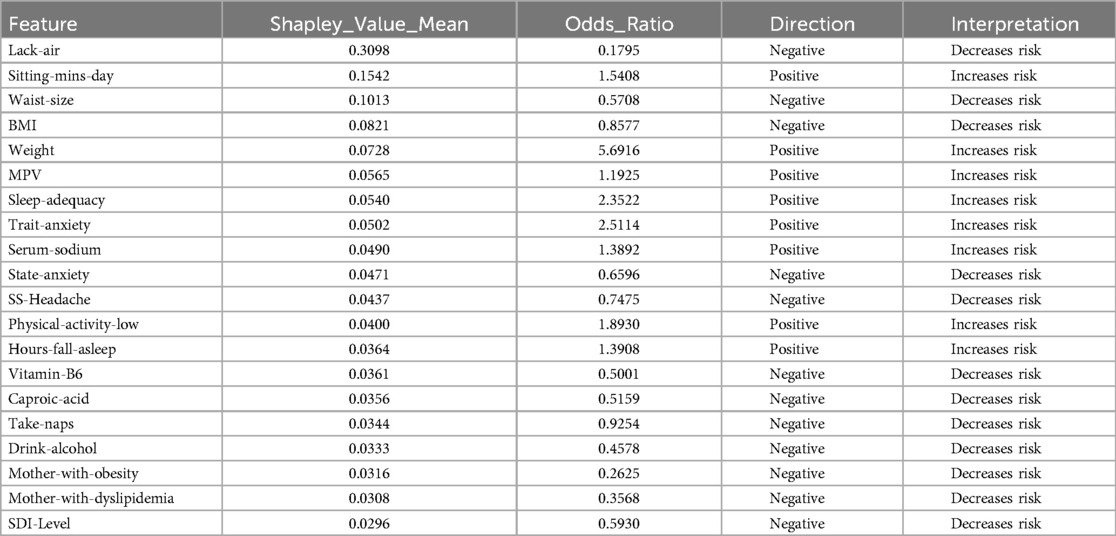
Table 1. Features obtained by XGBoost and SHAP using ADASYN.

In the results obtained with SVM using SMOTE technique (see Figure 3 and Table 2), Lack-air emerges as the most significant feature, evidenced by a high SHAP value and a large cluster of red points on the right side of the plot. Despite its high impact in SHAP, the odds ratio for Lack-air is 0.1845, indicating a decreased risk of hypertension for individuals with this feature. Other sleep-related variables, such as Hours-fall-asleep, Sleep-adequacy, Snores, Somnolence and Take-naps also play prominent roles, reflecting a strong association between sleep quality and hypertension risk.

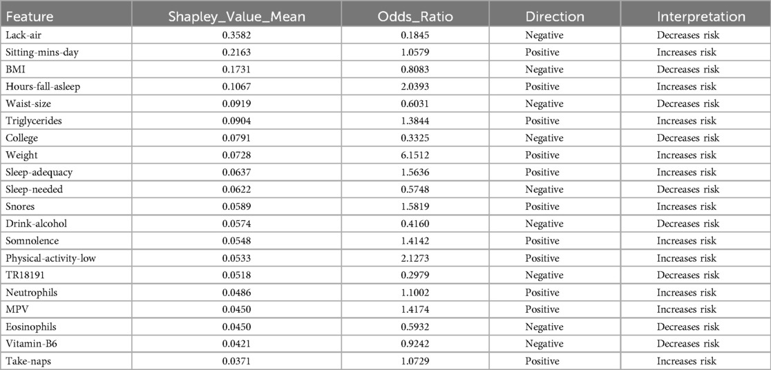
Table 2. Features obtained by XGBoost and SHAP using SMOTE.

Again in this model expected variables such as Sitting-mins-day, Low-physical-activity and Weight show a rightward spread, emphasizing the impact of sedentary behavior and obesity-related factors on hypertension, with high SHAP values and positive odds ratios indicating increased risk. Triglycerides, with a positive odds ratio of 1.3844, aligns with cardiovascular risk. Lower-ranking features such as Neutrophils, Eosinophils, and MPV also contribute positively, indicating their relevance in hypertension prediction.

In the case of features identified by SVM with ADASYN or SMOTE, they showed significant variations to compared to those in Figures 2 and 3. This discrepancy stems from the SVM models’ non-tree-based structure, prompting SHAP to adopt a permutation-based approach for calculating values, which typically yields a single SHAP value for each feature. In contrast, when using tree-based models such as XGBoost, SHAP utilizes TreeExplainer, a method specifically designed for these models. This approach facilitates the computation of detailed SHAP values for every feature, thereby offering a more nuanced depiction of how each feature impacts the model’s predictions.

The analysis using SVM and ADASYN (see Figure 4 and Table 3) identified features like Worker-unqualified, High-school, LDL-cholesterol, Cryptoxanthin, and C1S1891 as top predictors for the model of hypertension risk.

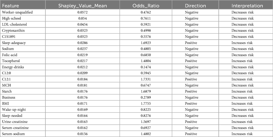
Table 3. Features obtained by SVM and SHAP using ADASYN.

Similarly, in the SVM analysis with SMOTE, key features such as College, Weight, Calcium, Worker-skilled, Soluble-fiber, and High-school show high SHAP values, indicating a strong impact on the model’s predictions (see Figure 5 and Table 4).

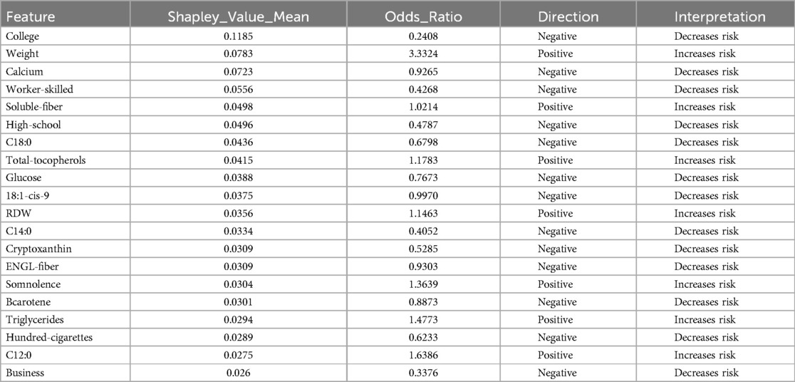
Table 4. Features obtained by SVM and SHAP using SMOTE.

Notably, although these features exhibited high SHAP values, their odds ratios were below 1, prompting further analysis to better understand their behavior across different algorithms.

In the ADASYN analysis, Urine-creatinine, Serum-sodio and Sleep-adequacy were found to have odds ratios significantly above 1, suggesting that these factors are closely linked to an increased hypertension risk. Their high odds ratios imply a more tangible and direct contribution to hypertension risk compared to features identified with high SHAP values alone.

For the SMOTE analysis, variables such as Weight, Somnolence, Triglycerides and others were marked by high odds ratios, making them essential to predict hypertension risk.

In summary, the comparative analysis of XGBoost and SVM using different balancing techniques and feature selection with Shapley Values demonstrates that the XGBoost model combined with SMOTE achieved the highest balanced accuracy at 90%, with a sensitivity of 0.8448 and a specificity of 0.9623 (see Table 5). This result indicates that the XGBoost-SMOTE configuration provides the best overall performance for hypertension prediction in this study, balancing the ability to correctly identify both positive and negative cases. Other models, including XGBoost with ADASYN and SVM with both ADASYN and SMOTE, also showed respectable performance but did not reach the same level of balanced accuracy.

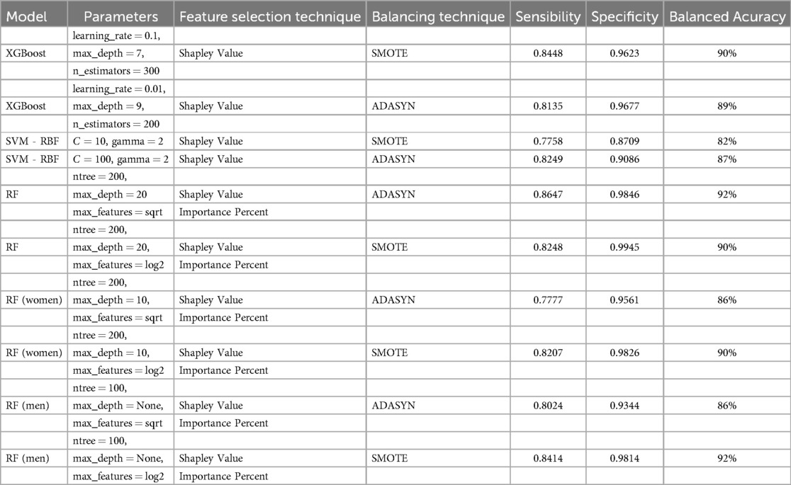
Table 5. Comparative performance of Machine Learning Models.

Given the results obtained, a further analysis was conducted using the Random Forest algorithm. Unlike the previous analyses, which utilized odds ratios to establish variable contributions, this approach applied the variable importance metric within Random Forest to identify the most significant features. To complement this, Average SHAP values were employed to determine the direction and contribution of each variable whether they increase or decrease hypertension risk. The choice to use SHAP values instead of odds ratios in this phase was intentional, as SHAP values are specifically designed to explain complex, non-linear models like Random Forest. Unlike odds ratios, which measure association strength in more linear contexts, SHAP values allow us to understand both the direction and the magnitude of each feature’s impact on individual predictions within a tree-based model.

3.2.2 Feature selection and contribution assessment using random forest

In this segment, we conducted an assessment of feature contribution using Random Forest and Shapley Values in combination with ADASYN and SMOTE (see Tables 6 and 7), evaluating both the importance of each feature and the direction of their influence on hypertension risk. Table 6 displays the results, detailing the RF Importance, average SHAP values, direction (positive or negative), and the associated impact (whether it increases or decreases hypertension risk). The direction and impact of each feature in predicting hypertension risk were determined through SHAP values, which offer insight into how each feature contributes to increasing or decreasing the model’s predictions.

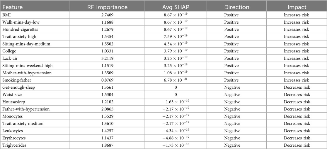
Table 6. Feature contribution using RF Importance, SHAP Value and ADASYN.