1 Introduction

In machine learning, unsupervised clustering has been widely discussed and applied. It refers to a data-analysis problem where the true classification of individuals (or items) is unknown, and we derive clusters by exploiting between-individual similarity. Clustering serves as an important tool for population stratification, image segmentation, anomaly detection, etc. (Ghosal et al., 2020). Specifically, clustering in medicine helps subgroup patients with potential disease risks and characterize each subgroup with distinctive genetic information. Patient subgrouping or disease subtyping plays an essential role in precision medicine, given that traditional medicine tends to offer a one-size-fits-all solution over the entire population and often overlooks heterogeneity (Spycher et al., 2008; Saria and Goldenberg, 2015). While designing a drug customized for every patient may not be feasible, fine-scaled disease subtyping is tractable and can facilitate more personalized prevention, diagnosis, and treatment.

To better characterize a disease or phenotype, it is beneficial to turn to different sources, i.e., multi-view data, that are jointly more comprehensive and informative than single modalities (Gligorijević et al., 2016). For example, prior work has shown that multi-view clustering algorithms often outperform single-view ones (Abavisani and Patel, 2018; Chauvel et al., 2020; Wen et al., 2021). However, many multi-view clustering methods have difficulty finding the consensus between modalities or exploiting relationships within and between views. Canonical correlation analysis (CCA) provides a solution to obtain optimal linear transformations of every data type to maximize their correlation (Hotelling, 1936). Moreover, sparse CCA (sCCA) introduces a sparsity parameter for each view, which can enforce the canonical weights on most features to be zero (Witten et al., 2009). sCCA both reduces the feature dimensionality and removes noisy features. Therefore, we can use this method to select the most meaningful features from datasets as input for the subsequent clustering. Sparse multiple canonical correlation network analysis (SmCCNet) can take an extraneous variable to detect modules of multi-view features with maximal canonical correlation between the data views informed by a phenotype of interest (Shi et al., 2019).

Current multi-view sample clustering methods integrate data views in different ways, e.g., concatenating all features, mapping views to a shared low-dimensional space, and merging between-sample relationship matrices from every view. The approach iCluster+ was designed to predict cancer subtypes from various data types by constructing a common latent space from all views (Mo et al., 2013). The extension iClusterBayes adopts a Bayesian model in the latent space (Mo et al., 2018). PintMF imposes a sparsity penalty on matrix factorization to integrate multiple data types into a common space (Pierre-Jean et al., 2022). Other state-of-the-art methods focus on combining similarity matrices from every data view. For example, Spectrum is such a method with a self-tuning density-aware kernel and similarity network fusion (SNF) that transforms data views to sample networks and fuses them nonlinearly (Wang et al., 2014; John et al., 2019). MRGC learns a robust graph for each data view and unifies them afterward (Shi et al., 2023). However, all the above-mentioned methods either reform the feature space or compute the between-sample interactions from features, which becomes deficient with data containing much information in the between-feature interactions.

Feature interactions derived from large sample collections are not individual-specific, although this has been shown to highlight interwiring modules for risk prediction and corresponding sample subtyping. Some analysis flows that illustrate this are built on the weighted gene co-expression network analysis (WGCNA) algorithm (Langfelder and Horvath, 2008). Starting from global networks, namely, networks built on a collection of samples, each individual’s perturbation to the global network can be used to derive a so-called individual-specific network or ISN (Kuijjer et al., 2019). Comparing ISNs thus implies comparing interaction profiles between individuals. In reality, different features contributing to individual wirings may have different origins, paving the way for system-level clustering of individuals in a precision medicine context.

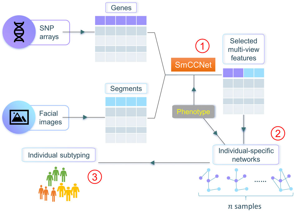
In this work, we propose netMUG (network-guided MUlti-view clusterinG), a novel multi-view clustering pipeline that clusters samples on the basis of these sample-specific feature interactions or wirings (Figure 1). In the presence of 2-view data, multi-view features are jointly selected via SmCCNet, based on canonical correlations and an additional extraneous variable. ISNs are constructed from the selected features, taking as a measure of edge strength the overall correlation between every pair of features and the extraneous data. The Euclidean distance metric representing dissimilarities between ISNs is fed into Ward’s hierarchical clustering (Ward, 1963), using the R library Dynamic Tree Cut to automatically derive the number of clusters (Langfelder et al., 2008). After validating netMUG on synthetic data, we applied our workflow to a collection of participants of recent European ancestry with both genotypic information and 3D facial images available (White et al., 2021). The aim was to dissect and interpret between-individual heterogeneity, informed by BMI as extraneous data. The application showed the potential of netMUG to refine existing classifications for obesity and to identify novel gene-BMI associations not yet discovered by genome-wide association studies (GWAS).

FIGURE 1. Workflow of netMUG (network-guided multi-view clustering). The pipeline consists of three parts: ① select phenotype-informed features from multiple data modalities via SmCCNet; ② build individual-specific networks based on the selected features and the phenotypic information; ③ subtype individuals via Ward’s hierarchical clustering.

Contributions of this paper:

• We developed a novel multi-view clustering method, netMUG, that combines feature selection, network construction, and downstream unsupervised learning in a single workflow.

• netMUG exploits the synergy between data views, as well as extraneous information, to assess heterogeneity between individuals and help in disease subtyping and stratified prevention.

• We simulated two data types whose features are cross-linked and whose samples have a complex clustering structure to validate the performance of netMUG.

• On a real-life dataset with genetic and facial information, netMUG informed by BMI as extraneous information highlighted known and novel characteristics of obesity.

2 Materials and methods

The code of netMUG is available on GitHub, along with its computational environment for reproducibility (https://github.com/ZuqiLi/netMUG.git). The complete pipeline, simulation, and analyses were done in R (version 4.2.1). The data representation of the case study was computed in Python (version 3.9.7).

For the remainder of this paper, we denote the two data views as X∈Rn×p and Y∈Rn×q, respectively; the phenotypic variable is Z∈Rn, where n is the number of individuals, p is the number of features in view 1, and q is the number of features in view 2.

2.1 SmCCNet

The SmCCNet pipeline consists of a sparse multiple canonical correlation analysis (SmCCA) and a module detection method (Shi et al., 2019). CCA and its variants are a set of multivariate statistical methods based on the cross-covariance matrix. The basic CCA aims to find a pair of vectors a∈Rp and b∈Rq that maximizes the correlation between Xa and Yb:

a∼,b∼=argmaxa,bcorrXa,Yb=argmaxa,baTΣXYbaTΣXXabTΣYYb(1)

where ΣXY denotes the cross-covariance matrix between X and Y, and ΣXX and ΣYY are the covariance matrix of X and Y, respectively. If we standardize both X and Y so that every feature has a mean of 0 and a standard deviation of 1, Eq. 1 can be reduced to

a∼,b∼=argmaxa,baTXTYbaTXTXabTYTYb(2)

If we further constrain the covariance matrices to be diagonal, Eq. 2 can be rewritten as

a∼,b∼=argmaxa,baTXTYb,s.t.a2=b2=1(3)

In case there are a lot of features with very little contribution to the canonical correlation, a sparse version of CCA (sCCA) is introduced, which applies the l1 regularization to the canonical weights a and b. Hence, the objective of sCCA is as follows:

a∼,b∼=argmaxa,baTXTYb,s.t.a2=b2=1,a1≤c1,b1≤c2(4)

where c1 and c2 are user-defined constants that regulate the sparsity, c1∈1,p, and c2∈1,q. Their values can be chosen via cross-validation.

CCA and sCCA are originally designed for only two data views; however, additional information may be available and it may be helpful to take into account the correlations between the existing views and the extra one. In the special case where the extra data type contains only a single feature, e.g. a phenotype of interest, this can be considered as finding the optimal canonical pair from the two existing views that also correlates with the phenotype. With the phenotypic variable denoted as Z∈Rn, the objective of SmCCA becomes

a∼,b∼=argmaxa,bw1aTXTYb+w2aTXTZ+w3bTYTZ,s.t.a2=b2=1,a1≤c1,b1≤c2(5)

Coefficients w1, w2, and w3 balance the three canonical correlations to account for the different correlation strengths among the multiple data types.

The pair of canonical weight vectors a∼,b∼ learned from the SmCCA are sparse indicators of how much every feature in X and Y contributes to the overall correlation among the two data modalities and the phenotype. If we concatenate a∼ and b∼ to form a new vector, ab∼, from which we can construct us a similarity matrix whose elements measure the relatedness between every two features:

where ⊗ is the outer product operator and ⋅ takes the absolute value of every element in a matrix.

To make the canonical weights robust, SmCCNet integrates a feature subsampling scheme, which results in multiple pairs of a∼,b∼ with different subsets of features from X and Y. The similarity matrices from each pair are then averaged and divided by the maximum.

Hierarchical clustering with complete linkage is performed on the distance matrix 1−S¯, where S¯ denotes the averaged and rescaled similarity matrix. The dendrogram is subsequently cut at the user-specified height and modules with feature(s) from a single view are discarded to derive multi-view modules.

2.2 netMUG: workflow and algorithm

The input of netMUG is multi-view data with a phenotype (or more generally, extraneous variables), both describing the same set of samples. To reduce dimensionality and extract the most informative features, netMUG first incorporates SmCCNet for feature selection, namely, features in the final modules detected by SmCCNet. We have found that in practice, it is difficult to assess and quantify the balancing weights on each pairwise correlation (see Eq. 5), so this property has been omitted in netMUG, i.e., w1=w2=w3=1.

We then use the selected features to construct ISNs for each individual. These networks are characterized by individual-specific edges as well as individual-specific nodes. In particular, we first construct a global network Gα=V,Eα across all samples, where V denotes the set of selected features from both views and Eα, the set of edge weights whose element eijα is the sum of pairwise Pearson correlations between feature i, j, and the phenotype Z on all samples:

eijα=corrVi,Vj+corrVi,Z+corrVj,Z(7)

Second, we compute the leave-one-out network Gα−s=V,Eα−s whose edges Eα−s are derived from all samples but sample s, similarly to Eq. 7. Intuitively, the difference between the global and leave-one-out networks measures the perturbation on the network caused by sample s. Based on this, in our work, we define ISN by the absolute differential network:

eijs=eijα−eijα−s for∀i,j∈1,2,⋯,r(8)

where eijs is the edge value between node i and j in the network specific to individual s. Hence, Gs=V,Es, and r is the number of selected features. Eq. 8 is a variant of the original ISN construction method reported by Kuijjer et al. (2019) because deriving an individual-specific association is not essential when the final aim is to identify “distances” between individuals. A higher eijs indicates that individual s deviates from its population more than others concerning the joint correlation between features and phenotype. In addition, an ISN with patterns that are very different from those of another ISN means that their corresponding individuals may belong to different population subgroups.

The edge weights in an ISN can be seen as the coordinates of a data point in a k-dimensional Euclidean space, where k = number of edges. Accordingly, clusters can be achieved by hierarchical clustering on Euclidean distance and Ward’s linkage. Because the Euclidean distance is not squared, we chose “ward.D2” as the method for the R function “hclust” to adopt the correct Ward’s clustering criterion (Murtagh and Legendre, 2014). The clusters are obtained automatically via the R package “dynamicTreeCut”, which iteratively cuts the hierarchical tree and determines the optimal number of clusters based on their shape. We set its hyperparameter deepSplit = 1 to have fewer but larger clusters.

2.3 Simulation study

We synthesized 1,000 samples with two views, each of which contains 1,000 variables, simulating complex, cross-linked datasets, e.g., genetic and facial data. Samples are randomly distributed in three balanced clusters. Because real-life data often contain a large number of uninformative features, we generated 600 variables of each data view from standard normal distribution N0,1, representing the noise. Then, the remaining 400 features were correlated within and between the two views to different extents by linearly transforming 400 orthogonal vectors per view.

The first 200 orthogonal vectors in each view, Xcorr and Ycorr, were sampled from a multivariate normal distribution with random covariance ranging from 0.5 to 0.8, i.e., Xcorr Ycorr∼N0,Σ, where Σ=IRRI, I∈R200×200 is an identity matrix, and R∈R200×200 is a diagonal matrix with the 200 covariances on the diagonal. The remaining 200 vectors in each view, Xclust and Yclust, were generated similarly but with covariance ranging from 0.8 to 1. Xclust and Yclust have three distinctive clusters of samples by multiplying 1, 2, and 3 by their values for the samples in every cluster. The clustering also gave rise to a phenotype that follows a different normal distribution in every cluster, i.e., Z=Z1 Z2 Z3T, where Z1∼N−1,1, Z2∼N0,1, and Z3∼N1,1. To make the correlation patterns more complex and representative of real-life data, we linearly transformed Xcorr Xclust and Ycorr Yclust by multiplying a square coefficient matrix whose values are random in the uniform range −3,3.

We also investigated the execution time spent by each model. The bottleneck of netMUG is the SmCCNet step that computes a full SVD internally for each dataset, whose time complexity is Omin⁡⁡mn2,nm2, where n and m are the two dimensions of the data matrix. To make the method applicable to large-scale datasets, e.g., the whole genomic data composed of millions of SNPs, we may replace the full SVD with truncated SVD in the future for much faster computation and less memory usage.

2.4 Case study2.4.1 Data representation

Data pre-processing resulted in 265,277 SNPs and 7160 3D facial landmarks for all 4,680 individuals with European ancestry (detailed steps are described in the Supplementary Material). We subsequently reduced the dimensionality of both genomic and facial data via principal component analysis (PCA) (Pearson, 1901). Specifically, SNPs were first mapped to protein-coding genes if they fell within 2000 base pairs around a gene. Genes mapped with less than three SNPs were removed for insufficient information. Then, we performed PCA on the SNPs in every gene to obtain the principal components (PCs) explaining at least 90% of its variance to represent each gene by fewer but more informative features. Meanwhile, we hierarchically segmented 3D facial images into five levels and 63 segments via the method proposed by White et al. (2021). Finally, the optimal number of PCs representing every facial segment was determined via the simulation-based parallel analysis. As a result, we obtained 60,731 PCs for 9,077 genes and 1,163 PCs for 63 facial segments.

2.4.2 Group-level interpretation

To estimate the association of BMI with our genomic data, we first conducted a GWAS via PLINK to calculate the p-value of the Wald test (detailed steps are described in the Supplementary Material), which would identify whether an SNP is significantly associated with BMI. Only SNPs with FDR-adjusted p-values <0.05 were kept and then mapped to genes, following the same mapping strategy as in the ‘Data representation’ step. Meanwhile, we also downloaded the list of BMI-relevant genes from the DisGeNET database with a decent filter (≥0.1) on the gene-disease association (GDA) score.

To further analyze the behavior of SmCCNet, we reran it with the same settings but without phenotypic information (the two sparsity parameters were re-determined via cross-validation). So far, four sets of genes have been obtained from the standard SmCCNet, GWAS, DisGeNET, and the uninformed SmCCNet. We investigated the overlap among them to see the agreement between SmCCNet and GWAS, the enrichment of DisGeNET genes in the gene set of SmCCNet (detailed steps are described in the Supplementary Material), and the difference in SmCCNet made by the presence of phenotype.

2.4.3 Cluster-level interpretation

We first evaluated the relationship between BMI and the clustering derived by netMUG. Namely, we conducted a Kruskal–Wallis test to determine whether there were statistically significant differences in BMI distributions among the clusters. Our obesity subtypes were also compared with the classic BMI categories, i.e., underweight (BMI <18.5), normal (18.5≤BMI <25), overweight (25≤BMI <30), and obese (BMI≥30) (WHO Global InfoBase team, 2005).

Further, we characterized every subgroup by facial and genetic information. By averaging all facial images of each subgroup, we represented it with a mean face shape. As for genetics, ISNs of every cluster were averaged, and a subnetwork was taken from the mean ISN based on the top 1% edge weights to only focus on the vital signals. Subsequently, we computed the largest connected component of every subnetwork and extracted all genes in this component. The overlap among clusters was analyzed, and we paid special attention to the cluster-specific genes to characterize each cluster. In particular, an enrichment analysis was done via the analysis tool of the Reactome website (Gillespie et al., 2022) to test which biological pathways are significantly over-represented in the gene list specific to every cluster.

2.4.4 ISN-level interpretation

Because our pipeline represents every individual by a network, namely, ISN, a fully-connected weighted graph, we need a lower-dimensional representation of the ISNs to examine their behavior better and visualize them. Therefore, the graph filtration curve method was applied, which computed a function or curve from each ISN, whose values were derived via graph evolution (O’Bray et al., 2021). More specifically, we set a series of thresholds on the edge weights and, at each threshold, constructed a subnetwork by taking only edges larger than that threshold. In such a manner, we got a series of subnetworks from smallest to largest for every ISN, and the largest subnetwork is the ISN itself. Then, graph property was calculated based on each subnetwork, and therefore, an ISN was converted to a function of graph property against the edge threshold. Here, in our project, we chose the mean node degree of the largest connected component (LCC) as the graph property because the subgraphs may not be fully connected anymore. The average degree is a simple yet powerful tool to measure graph density.

3 Results

netMUG was validated on a synthetic dataset and compared with both baseline and benchmark methods for multi-view clustering. We then applied it to real-life large-scale multi-view cohort data and characterized the resultant clusters by their representative faces and enriched pathways.

3.1 Validating netMUG on synthetic data

We simulated a scenario where a multi-view dataset contained complex feature patterns and many noisy features, representing real-life high-dimensional data, e.g., genomics and images. Two criteria were adopted to assess clustering performance, p-value from the Kruskal–Wallis test, and adjusted Rand index (ARI). The Kruskal–Wallis test was used as a non-parametric version of one-way ANOVA to test whether the distribution of an extraneous phenotype is similar across clusters because the simulated phenotype follows a multimodal distribution (Kruskal and Wallis, 1952). Therefore, a low p-value (<0.05) indicates a significant association between the clustering and the phenotype. ARI was computed to show the similarity between the derived clustering and the phenotype (Rand, 1971): the higher, the better; an ARI of 1 means perfect fitting.

Various baseline and benchmark methods were considered in addition to netMUG, and their performances were compared. Baseline models included k-means on every single view, and both views concatenated, with or without principal component analysis (PCA) as a data dimensionality reduction strategy. We chose four benchmark models, iCluster+ (Mo et al., 2013), iClusterBayes (Mo et al., 2018), Spectrum (John et al., 2019), and SNF (Wang et al., 2014), and their codes are available in R (R Core Team, 2022). To show the effectiveness of SmCCNet as a feature selector, we also applied Spectrum and SNF on the features selected by SmCCNet, i.e., model “SmCCNet-Spectrum” and “SmCCNet-SNF’. Finally, as an alternative to our proposed framework, we replaced hierarchical clustering with spectral clustering as the last step of netMUG, leading to the model ‘SmCCNet-ISN-SC’.

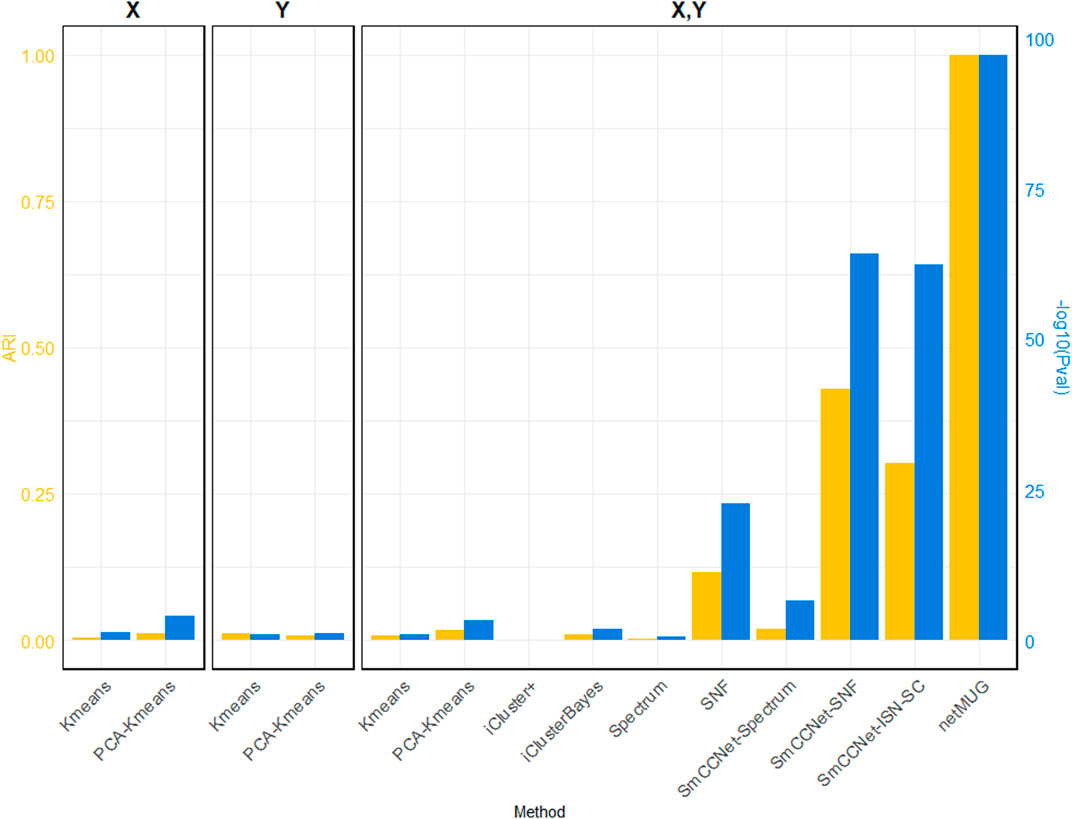
As shown in Figure 2 (exact values are listed in Supplementary Table S1), all baseline models performed poorly in terms of ARI. The p-values for models with PCA on single X and both views were lower than 0.05 but did not convey a big difference on the plot. Among the benchmarks, SNF outperformed iCluster+, iClusterBayes, and Spectrum. With features selected by SmCCNet, the performances of both Spectrum and SNF were substantially improved, implying the necessity of feature selection on high-dimensional and noisy data. Integrating SmCCNet, ISN, and Dynamic Tree Cut, netMUG achieved the best p-value and ARI results. It retrieved the clustering of phenotype for the complex multi-view data we simulated.

FIGURE 2. Performance of all methods on simulated data. The three barplot panels illustrate the ARI (on the left axis in yellow) and −log10Pval (on the right axis in blue) for the 4 single-view (X or Y) and 10 multi-view (both X and Y) models. Four out of six baseline models (“Kmeans” and “PCA-Kmeans”) use a single view (X or Y). Two-view “Kmeans” and “PCA-Kmeans” models are based on the concatenation of X and Y. “SmCCNet-Spectrum” and “SmCCNet-SNF” are benchmark models with features selected by SmCCNet. “SmCCNet-ISN-SC” only differs from the proposed framework, netMUG, for the clustering method.

The runtime of each method (Supplementary Table S1) shows that all baseline models spent less than half a minute and PCA brought an acceleration in speed for fewer features. iCluster+ and iClusterBayes spent much more time than Spectrum and SNF, without an improvement in performance. The SmCCNet feature selection step took 33 min on its own, which became the bottleneck of all the SmCCNet-based models (‘SmCCNet-Spectrum’, ‘SmCCNet-SNF’, ‘SmCCNet-ISN-SC’, and netMUG). This is mostly due to the subsampling scheme and the full SVD computation within SmCCNet.

3.2 Case study

To exemplify netMUG, we used a multi-view dataset of 4,680 individuals of recent European ancestry recruited from three independent studies in the US: 3D Facial Norms cohort (PITT), Pennsylvania State University (PSU), and Indiana University-Purdue University Indianapolis (IUPUI) (White et al., 2021). For each individual, facial images and genomic data were collected along with extra information, including age, sex, height, and weight. BMI was computed as BMI=weightkg/heightm2. Because both facial and genomic data are high-dimensional, we converted them separately into low-dimensional PC spaces before feeding them into a netMUG pipeline. More specifically, the genomic and facial data views had 60,731 and 1,163 PCs as features, respectively.

We interpreted netMUG analysis results at two levels: at the all-samples level, hereafter referred to as “group-level”, and at the level of clustered individuals. Group-level interpretation refers to describing the multi-view features selected by SmCCNet. In addition, we assessed the overlap between SmCCNet-selected genes and genes found by a genome-wide association study (GWAS) or DisGeNET database. Cluster-level interpretations were made by evaluating the association between the final clustering and BMI and the characterization of every cluster in terms of facial or genetic characteristics. Finally, we applied graph filtration curves to represent and visualize ISNs in 2D space (O’Bray et al., 2021).

Two flavors of netMUG were implemented: one with SmCCNet informed by BMI as an extraneous variable, and one without such information.

3.2.1 Group-level interpretation

Informed by BMI. We chose the two sparsity parameters for SmCCNet, namely, c1 and c2 in Eq. 5, via 5-fold cross-validation, predicting the canonical correlation. The subsampling proportions were determined as 50% and 90% for genomic and facial data because of their substantial dimensional differences. We then computed the average canonical weights over 500 subsampling runs to derive the similarity matrix S¯. Three modules with 316 PCs (see Methods “Data representation”) were found by cutting the hierarchical tree at a height very close to 1 (0.999) and discarding modules with a single feature or features from a single view. The cutting threshold was determined following Shi WJ et al. (Shi et al., 2019). The selected features from the retained modules comprised 278 genes and 26 facial segments. All the subsequent analyses were performed on these features unless mentioned otherwise. One of the most well-known obesity-related genes, FTO (Fawcett and Barroso, 2010), was on the gene list. Another essential gene for obesity, MC4R (Loos et al., 2008) was not selected because it was filtered out for having less than three SNPs mapped. A recent epistasis analysis found two pairs of SNPs whose interactions were associated with BMI (FTO–MC4R and RHBDD1 – MAPK1) (D’Silva et al., 2022). SmCCNet did not detect RHBDD1 or MAPK1, possibly caused by CCA’s focus on inter-modal rather than intra-modal interactions.

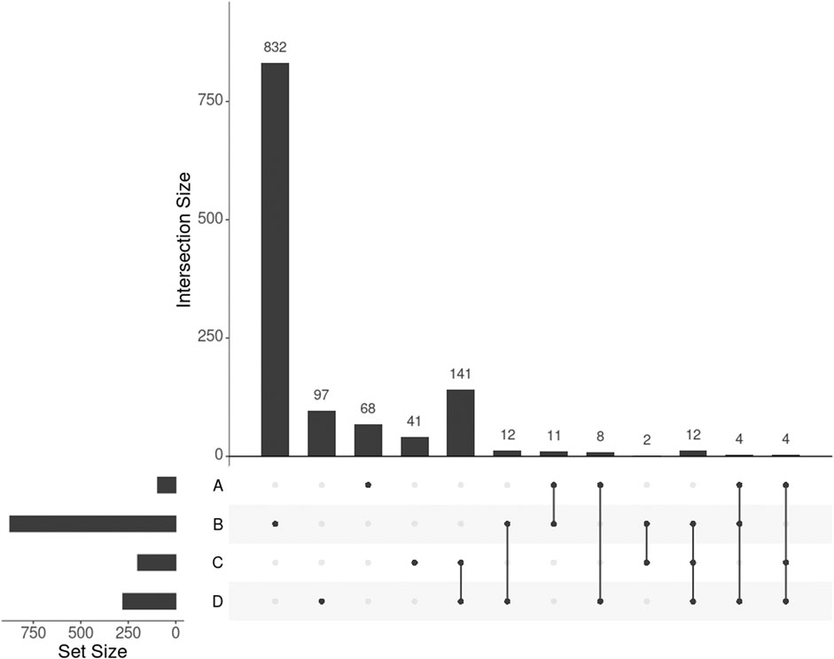
GWAS detected 155 SNPs significantly associated with BMI mapped to 95 protein-coding genes (p-value <0.05 adjusted by false discovery rate, or FDR). Out of these 95 genes, 16 (16.8%) were in common with the 278 genes selected by SmCCNet (Figure 3, set A and D), confirming the agreement between SmCCNet and GWAS but also explaining their differences in the involvement of facial information.

FIGURE 3. UpSet plot showing the intersections of four gene sets. A, B, C, and D represent the gene list found by GWAS, DisGeNET, uninformed SmCCNet, and standard SmCCNet, respectively. Uninformed SmCCNet maximizes the canonical correlation without extraneous information, whereas standard SmCCNet takes BMI into account to supervise CCA. Genes of the four sets are listed in the Supplementary Material.

We found 1,014 genes from DisGeNET associated with BMI with a gene-disease association (GDA) score≥0.1 (Piñero et al., 2019), of which 873 were protein-coding genes. Of the 873 genes, 28 (3.2%) also appeared in the 278 genes selected by SmCCNet (Figure 3, set B and D). The hypergeometric test showed that the DisGeNET gene set was significantly enriched in the gene set from SmCCNet (p-value = 6.0×10−5).

Uninformed by BMI. A total of 329 features were selected by the uninformed SmCCNet, resulting in 200 genes and 50 facial segments. Of the 200 genes, 157 (78.5%) were shared between the standard and the uninformed SmCCNet (Figure 3, set C and D). However, the uninformed SmCCNet found fewer GWAS genes (4) and DisGeNET genes (14) than informed SmCCNet (Figure 3, set A, B, and C). Furthermore, a lower percentage of BMI-related genes were selected by uninformed SmCCNet (2% in GWAS and 7% in DisGeNET) than informed SmCCNet (6% in GWAS and 10% in DisGeNET), highlighting the merits of supervised analysis.

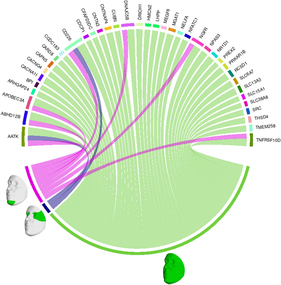
We also looked at the top 1% of connections between genes and facial segments in the features selected by informed SmCCNet (Figure 4). It was clearly shown that the full face has high relatedness with all genes, indicating that those genes are primarily associated with facial morphology globally. On a local level, the selected genes are most strongly connected with the eyes (with the temporal area) and chin, in line with the fact that they are known facial signals of obesity. AATK and CD226 are the genes with the most top connections. AATK plays a role in neuronal differentiation and has been known to be highly associated with BMI (Zhu et al., 2020). CD226 encodes a glycoprotein expressed on the surface of blood cells and is related to colorectal cancer (Storojeva et al., 2005), which could be a potential biomarker of obesity. Furthermore, APOBEC3A, DNAJC5B, and NGFR all affect body height and BMI (Kichaev et al., 2019).

FIGURE 4. Genes and facial segments with the top 1% connections. Connections refer to the similarities between the canonical weights of genetic and facial PCs, as described in Methods. Only inter-modality relationships are considered. A thicker connection in the circus plot means a higher relatedness.

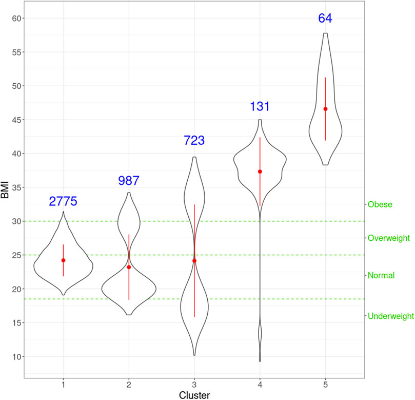
3.2.2 Cluster-level interpretation

netMUG automatically detected five clusters with significantly different BMI distributions given the Kruskal–Wallis test (p-value = 7.4×10−150) (Figure 5). The derived clustering is much more significantly associated with BMI than the clustering uninformed by BMI (p-value = 1.8×10−17). Clusters 4 and 5 are the two outstanding subgroups, and both fall into the classic category of ‘obese.’ (WHO Global InfoBase team, 2005). Nevertheless, as clearly shown in Figure 5, our clustering provides higher granularity on the obese subgroup, which is desired because it can lead to more precise identification and better characterization of obese people. Cluster 1 contains roughly half the people in the dataset, and it substantially follows the distribution of the whole population with most normal and normal-to-overweight individuals. Clusters 2 and 3 have similar bimodal distributions with different deviations. The two peaks of cluster 3 are further away from the center than cluster 2. Jointly looking at clusters 1, 2, and 3, they classify individuals by how far they are from the ‘population normal’ while treating underweight and overweight indifferently. This behavior suggests that underweight and overweight people deviate from the normal condition similarly in terms of multi-view interactions, which may be related to, e.g., the double burden of malnutrition. It has been shown that some crucial vitamins and minerals can affect both underweight and overweight individuals.

FIGURE 5. Violin plots for the distribution of BMI for individuals in every cluster. For each cluster, the red dot and vertical line indicate the mean and standard deviation, respectively, and the number in blue is the size of every cluster. The three green horizontal dashed lines represent the cut-offs of the four classic BMI categories shown on the right Y-axis.

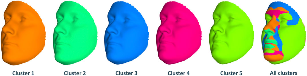
Next, we look at the genetic and facial characteristics of the identified clusters. The average facial shapes per cluster are depicted in Figure 6 and largely follow the profile of mean BMI across clusters (Figure 5). Again, clusters 4 and 5 stand out compared to clusters 1–3. Superposition of the average faces shows pronounced areas on the forehead or the chin for cluster 4 individuals, whereas cheek and eye areas are most responsible for cluster 5 differences in the rest of the samples. Cluster one to three faces have pronounced features around the nose and mouth.

FIGURE 6. Mean facial shapes of every cluster and the superposition of them. The first five faces are the average of all individual faces in every cluster, while the last face was obtained by plotting the five mean faces on top of each other (colors of this superposition face correspond to the five mean faces).

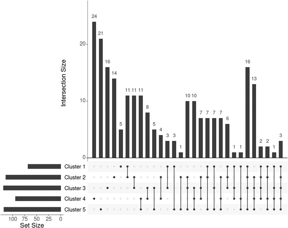
For individuals within every cluster, we averaged their corresponding ISNs and binarized the mean ISNs, with the top 1% edge weights being 1 and the rest 0. Subsequently, we computed the largest connected component (LCC) from every binary network, resulting in LCCs of 86, 129, 144, 112, and 136 nodes (68, 114, 119, 94, and 118 genes) for the five clusters, respectively (Figure 7). The genes MIGA1, CACNA1B, and SLC38A8 were common to all clusters. MIGA1 regulates mitochondrial fusion and shows a strong relationship with BMI according to the GWAS Catalog (scoring 14.0) (Zhu et al., 2020). CACNA1B encodes a voltage-gated calcium channel subunit and GWAS Catalog records a strong association (scoring 12.2) between CACNA1B and acute myeloid leukemia (Lv et al., 2017), for which BMI is a known risk factor. SLC38A8 has a high GWAS Catalog score (14.1) with adiponectin measurement (Spracklen et al., 2019), which directly affects insulin sensitivity and obesity, and a strong association with eye diseases, e.g., foveal hypoplasia 2 and anterior segment dysgenesis. The link from gene SLC38A8 to both obesity and facial features may imply a novel relationship between obesity and facial morphology.

FIGURE 7. UpSet plot showing the intersections of genes extracted from the mean ISN of every cluster.

To further investigate the genes exclusively extracted from each subgroup, i.e., subtype-specific genes, cluster 4 has the most subtype-specific genes (24) and also has the highest proportion (25%) of all the genes in its LCC, followed by cluster 5 with 21 unique genes (17.8%). This observation is in line with the distinctive BMI distributions for these clusters. Meanwhile, there are only five genes specific to cluster 1 (7.4% of 68 genes in the LCC of cluster 1), suggesting that cluster 1 represents the “population normal.”

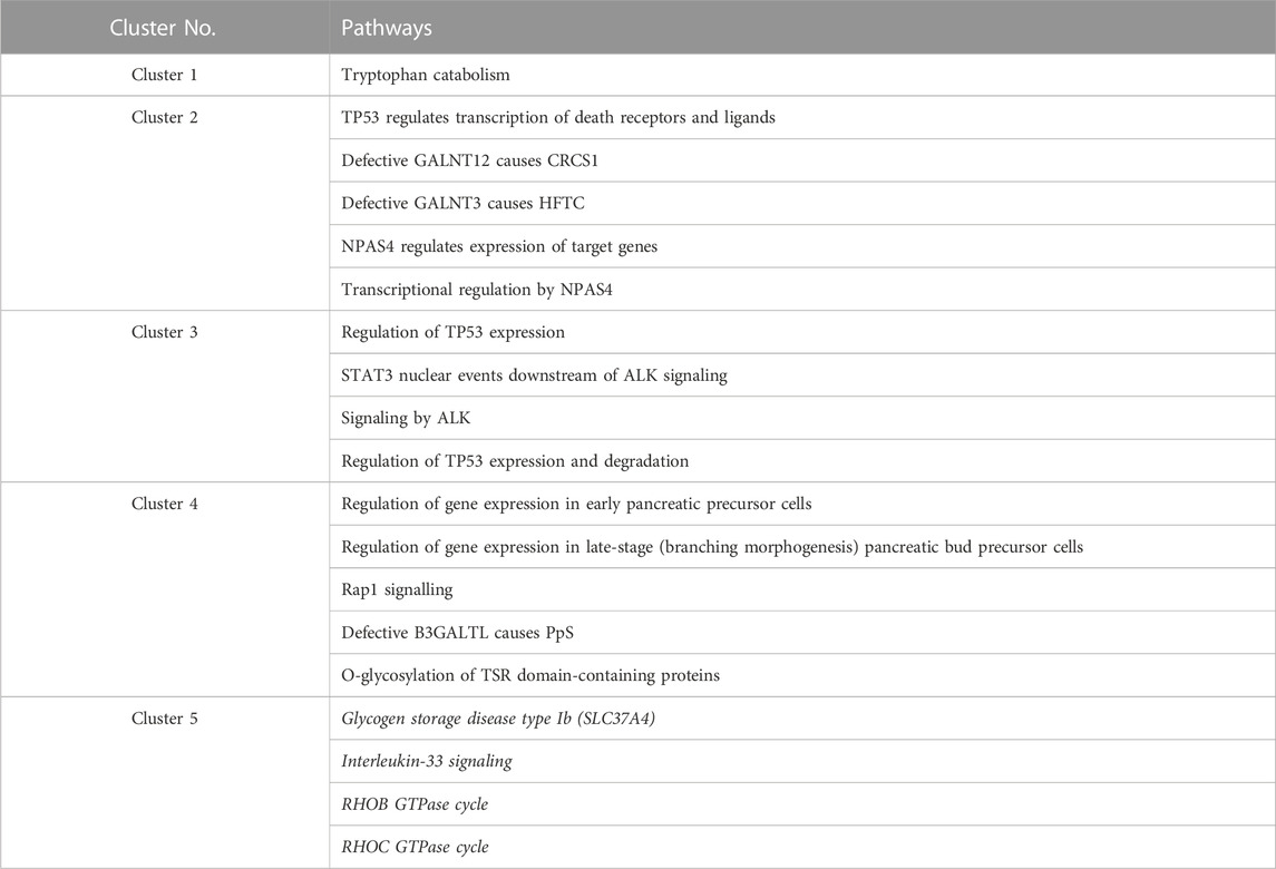
One or more Reactome pathways were significantly enriched in genes that were specific to a cluster, except for cluster 5 (Table 1). The reason may be that genes enriching cluster 5 were also obtained in other clusters, so they were not considered specific to cluster 5. Another possibility is that those 21 genes exclusively in cluster 5 are too functionally diverse as obesity is involved in many different biological pathways.

TABLE 1. Enriched Reactome pathways in every cluster. Pa