
Remember me
Radiomics, that is, the combination of automated, quantitative image analysis combined with machine learning (ML), allows for the prediction of clinical end points such as diagnosis or survival time from imaging data. Such an analysis typically comprises segmentation of the area of interest, followed by the calculation of a potentially large number of image properties, often referred to as “radiomics features”1 and can be viewed as the conversion of imaging data to structured, tabular data.2
Most radiomics studies in the literature are retrospective and of exploratory nature. Without a rigorous statistical analysis, the complexity and the multitude of configuration options in a radiomics pipeline might often lead to overly optimistic performance estimates. Combined with the fact that editorial policies often encourage the publication of positive findings, this may lead to a strong publication bias in the literature, which has been confirmed in a recent meta-analysis.3
Machine learning–based end point prediction from such tabular data requires setting up an analysis pipeline and involves numerous choices, which may include data set composition, feature selection,4 dimensionality reduction, selection of an ML algorithm, and their hyperparameter optimization (HPO).5 Often, these choices are based on expert knowledge, intuition, or simple performance metrics. In contrast, benchmark studies6 build the basis for objective comparisons of pipeline variations and are typically evaluated via nested cross-validation (CV) ensuring robust and (almost) unbiased performance estimations.7–9
To measure the effect of the experimental setup on the target metric and to identify the optimal pipeline configuration, a linear modeling approach is suitable. A linear mixed model (LMM) is recommended by Eugster et al10 to account for the repeated performance estimation of each pipeline configuration, each on the same train/test folds resulting from the used resampling strategy, for example, CV. This approach accounts for the interdependency11 of the benchmark results and allows for valid inference12 with respect to predictive performance.
Colorectal cancer (CRC) is the second most common cancer for women and the third most for men.13 Worldwide, it is the second leading cause of cancer deaths.14 The liver is the primary site of the metastatic disease, and consequently, the remaining liver function is an important factor for the survival of patients. Next to clinical and laboratory parameters describing liver enzymes and function, for example, albumin, alkaline phosphatase, neutrophil-to-lymphocyte ratio, and bilirubin, image morphological information from the whole liver, as well as the metastases, can be used for prediction of overall survival (OS).
The objective of this study was to develop a comprehensive ML pipeline for radiomics-based analyses, specifically for predicting OS in patients with intrahepatic metastases of CRC. We present a mixed model approach to identify the optimal pipeline configuration and evaluate the prognostic value of clinical features, compared with radiomics features derived from the whole liver, and intrahepatic metastases on computed tomography (CT) images.
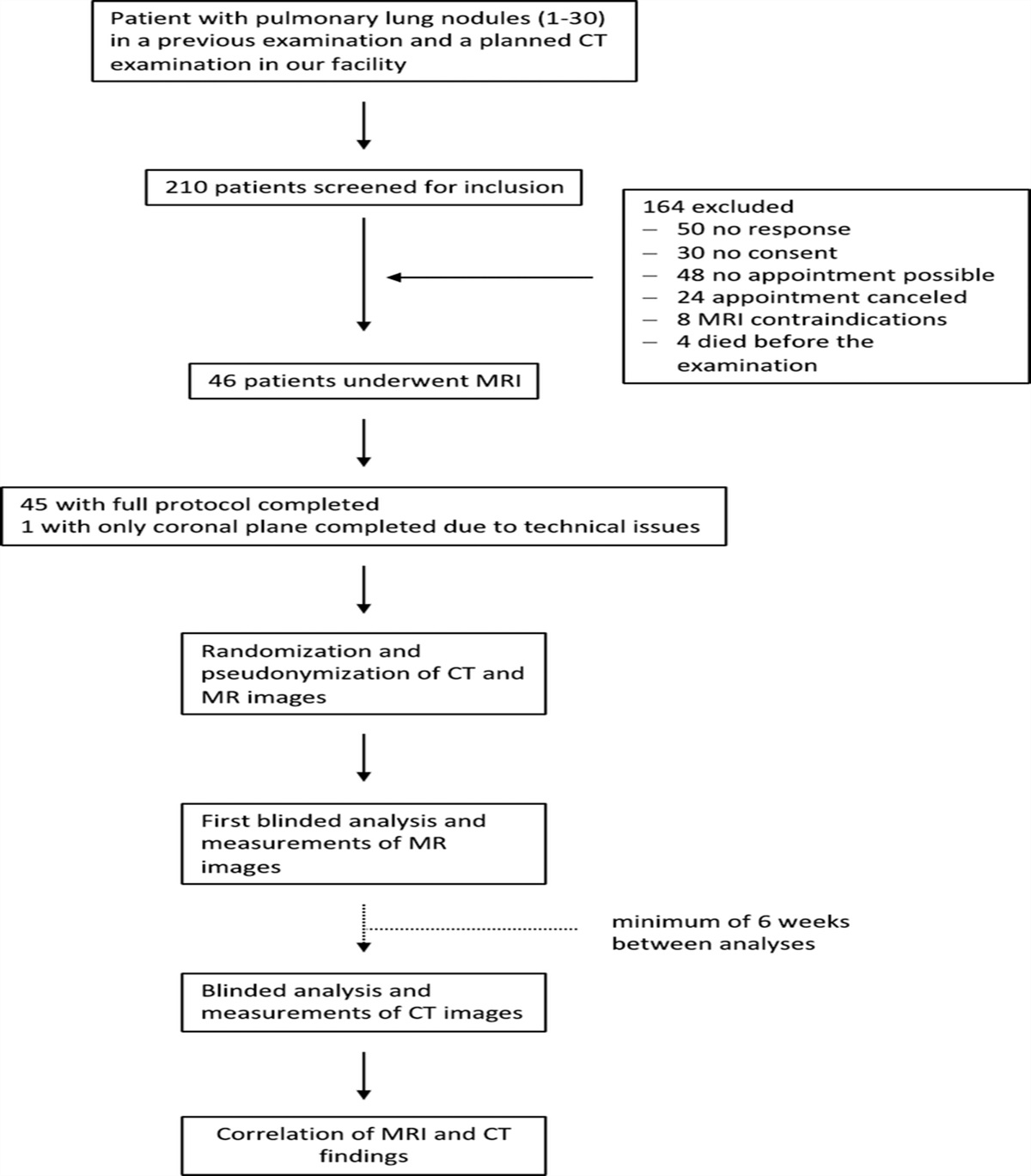
MATERIALS AND METHODS Patient Population and ImagingIn this study, we performed a retrospective analysis of data from a former prospective, randomized, multicenter SIRFLOX (Clinical Trails ID: NCT0072450315) trial.16,17 As a follow-up study, we analyzed OS with all-cause mortality. Our experiments are based on axial, contrast-enhanced CT images in the portal-venous phase, which were available for 491 of the originally 530 patients with intrahepatic metastases of CRC (Fig. 1). Two hundred thirty-nine of these patients received exclusively a standardized treatment, whereas 252 patients additionally received radioembolization with yttrium-90 (selective internal radiation therapy). Besides imaging and treatment data, supplementary clinical information was available and is summarized in Table 1. For further details, we refer to the original analyses.16,17
 FIGURE 1:
 Study flowchart. For 491 of the 530 patients, computed tomography (CT) imaging data were available for the study at hand.
TABLE 1 - Descriptive Statistics for Demographic, Laboratory, and Clinical (n = 491) Characteristics of Patients With Metastatic Colorectal Cancer No Variable Statistical Characteristics Frequency of Valid Values Valid Values Missing 1 Age in years (numeric) Mean (SD): 62.2 (10.7); min < med < max: 28 < 63 < 83; IQR (CV): 14 (0.2) 52 distinct values 491 (100.0%) 0 (0.0%) 2 Sex (factor) 1. FemaleComputed tomography images were rescaled to 1 × 1 × 1 mm3 isotropic spatial resolution, and liver and intrahepatic metastases were segmented using the pretrained nnU-net.18 For 80 randomly selected data sets, liver and liver metastases were manually segmented by an expert reader with 8 years of experience in abdominal radiology. Segmentations by nnU-net were evaluated against this reference standard by calculating the Dice scores for segmentations of liver and metastases. A detailed description can be found in the image preprocessing section in the Supplemental Digital Content, https://links.lww.com/RLI/A843.
Quantitative image features were calculated for whole-liver and tumor segmentations using the Python package PyRadiomics (version 3.0.1).1 Features characterizing the shape of the segmented volumes of interest were calculated on each of the segmentations. Furthermore, the images were preprocessed by 8 wavelet filters and 5 LoG (Laplacian of Gaussian) filters (1 mm to 5 mm), generating additional features for each filter separately in addition to the unfiltered original ones. On the volume of interest of these original and filtered images, features based on their gray-level distribution and texture, using matrices with gray-level bins of 25 HU (Hounsfield units), were calculated. In total, 1218 features were derived from each segmentation.
Importantly, features were calculated from 1 segmentation comprising all metastases in the liver. More precisely, 1 patient normally has multiple, segmented intrahepatic metastases, which we handled as 1 observation with respect to the on-patient-level prognosis. This especially affected the calculation and consequently interpretation of the shape-based radiomics features.
Machine Learning BenchmarkThe benchmark experiment was implemented in R (version 4.2.2)19 using the mlr3 framework,20 where also most of the terminology is derived from. This framework is schematically presented in Figure 2A and Figure 2B, and explained in the following subsections. The section Benchmark Setup of the Supplemental Digital Content, https://links.lww.com/RLI/A843, comprises an in-depth description of the construction details.
 FIGURE 2:
 A, Setup of the benchmark pipeline for the analysis of prognostic information in different (radiomics) feature sets regarding overall survival in patients with hepatic metastases due to colorectal cancer. The basis of the machine learning pipelines is given by the 3 algorithms—a random survival forest (RSF), a regularized generalized linear model (glmnet), and a gradient tree-boosting technique (xgboost)—combined with varying configurations of preprocessing (feature selection, principal component analysis yes/no) and tuning yes/no, evaluated with respect to the performance metric integrated Brier score (IBS). B, Detailed look into the tuning (k = 5)/performance (k = 10) loop for k-fold cross-validation (CV). Preprocessing steps in the pipeline construction and the corresponding learner development are based on the training folds, whereas model evaluation is based on the test fold.
Data Set ConfigurationThe predictor variables comprised the 3 groups: (1) clinical data, (2) image features derived from the whole liver, and (3) image features derived from intrahepatic metastases. Benchmarks were performed for every group and for the combinations of clinical data with each image feature group. These 5 configurations are further referred to as data sets.
Algorithms/LearnersA variety of ML models for survival analysis are available in mlr3proba.21 This study focused on a regression learner with elastic net regularization (glmnet22), a random survival forest (RSF23), and a tree-boosting algorithm (xgboost24).
Hyperparameter TuningThe performance of each learner was evaluated with and without HPO. Corresponding hyperparameters, their default settings, and search space can be found in Table S.1.1, Supplemental Digital Content, https://links.lww.com/RLI/A844. Tuning was performed only for the most relevant hyperparameters, which were selected in accordance with Probst et al25 and Bischl et al.5 Because of the amount of hyperparameter configurations and their possible combinations for the RSF and xgboost, hyperband tuning was used with the number of trees/boosting iterations as budget parameter to avoid wasting computational resources.26 In contrast, for the pipelines incorporating the glmnet, we only needed to tune a single hyperparameter, for which we used a random search strategy.
ResamplingTo ensure a robust training and evaluation process (outer), we selected stratified 10-fold CV as resampling method. For tuning, an inner 5-fold CV was invoked to determine the optimal hyperparameter configuration via nested CV, as illustrated in Figure 2B.
Feature PreprocessingWe included 4 preprocessing steps into a benchmark pipeline: (1) feature encoding (if needed), (2) imputation (if needed), (3) feature selection (optional), and (4) dimensionality reduction via principal component analysis (PCA) (optional). These preprocessing steps were performed in each inner and outer fold separately to ensure that information from the test set is not inadvertently used during training (data leakage), leading to overly optimistic results.
Feature selection—more precisely feature filtering—methods in step 3 were only investigated if the pipeline configuration included tuning. In this case, the filter with the best performance along with the according hyperparameter setting was automatically selected from 4 possible options: no feature selection, correlation-based feature filter, information gain filter, or selection via permutation importance of an RSF.27 The only hyperparameter tuned for all filter methods was the fraction of selected variables, ranging from 10% to 90% (see Supplemental Table S1.2, https://links.lww.com/RLI/A844). The last option in the preprocessing section was the performance evaluation with and without step 4 dimensionality reduction via PCA,28 where only the principal components of those features accounting for 90% of the variance were kept.
MetricFor HPO and the final model evaluation, we used the (restricted) integrated Brier score (IBS)29–31 performance metric. In absence of censoring, the Brier score (BS) is defined as the squared deviation of the estimated survival from the observed survival probability at time point t. When censored observations are present, BS is reweighted with the probability distribution of being censoring-free until this time point t. Integrated Brier score measures the inaccuracy for all available time points by integrating over the reweighted BS from t1 to tmax.21,32,33 Accordingly, lower IBS values indicate better performance. To overcome the overweighting of long survival times, integration was only done up to the 80%-quantile of the survival times instead of integrating over the whole follow-up time.34 For more details, see the according subsection in Benchmark Setup and Supplemental Eq. 1, Supplemental Digital Content, https://links.lww.com/RLI/A843.
Computational AspectsThe described benchmark experiment was run on a high-performance computing Linux Cluster from the Leibniz-Rechenzentrum. The main objective of the computational investigations was to determine if the time spent on tuning is justifiable based on the performance improvement achieved. Therefore, we report the median (outer folds) runtime of each combination of data set and pipeline composition separately for tuning and no-tuning settings. Computation times should not be directly compared between different learners due to variations in hyperparameters and search strategies. The reported run times are only meant for comparing tuned and untuned pipelines within each learner composition. Especially while the RSF and xgboost have built-in parallelization, we did not parallelize the automatic lambda search within the (CV-) glmnet.
Statistical Analysis Descriptive Benchmark AnalysisWithin our benchmark experiment, 60 different combinations of 5 data sets (clinical data; radiomics features of liver and tumors; combination of clinical and radiomics features) and 12 ML pipeline configurations (3 learners glmnet, RSF, and xgboost × 2 tuning options yes/no × 2 PCA settings yes/no) were evaluated. The resulting IBS performance values from the 10-fold CV were analyzed via boxplots arranged in grids of algorithm and preprocessing/tuning combination. Within the plots, points represent the exact IBS value obtained in each outer CV fold.
Mixed Model ApproachFor the meta-analysis of the benchmark results, we used an LMM,35 which combines fixed and random effects, to find significant differences between the observed performances. To allow this sort of inference12 with respect to the experimental benchmark setup, we incorporated the data sets and pipeline variations, together with their interactions as fixed effects into the LMM. We investigated the relevance of each fixed effect within the model via the analysis of variance.36
The random effect accounted for the correlation in the data induced by repeatedly using the same CV train/test sets for all ML pipelines.10,37 The necessity of the random effect was investigated visually and via the intraclass correlation (ICC). The ICC served as a measure for the variability between the CV groups, or conversely, the similarity within these groups (homogeneity) by returning the proportion of variance explained through this grouping factor.38,39 A schematic illustration of the LMM composition can be found in Figure S2 (https://links.lww.com/RLI/A846) and the corresponding mathematical formulation in Supplemental Eq. 2, each in the Supplemental Digital Content, https://links.lww.com/RLI/A843. The variance components of the LMM were estimated via (restricted) maximum likelihood optimization,35 and the model assumptions were checked (see Fig. S3, Supplemental Digital Content, https://links.lww.com/RLI/A847).
Mixed Model EvaluationA standard method for the evaluation of LMMs or especially the fixed effects is coefficient/dot-whisker plots40 along with Tukey contrasts.41,42 For our analysis, the effects were not readily comparable in this way due to the amount of pairwise combinations given by the interaction effect data set × pipeline. Instead, we calculated the estimated marginal means (EMMs; or least-squares/predicted means), which represent the mean of each predictor adjusted for the mean of the predictor(s) they interact with, in the model.43,44 These predictions were presented in an interaction-style plot45 containing the EMMs and their simultaneous confidence intervals (CIs).46,47
RESULTS Patient Population and ImagingFor our study, a collective of 491 patients with hepatic metastases abdominal CT scans were available from the original SIRFLOX study. The median follow-up was 57.2 months (interquartile range [IQR], 36.2–89.1). Four hundred seven of the 491 patients died (all-cause mortality) within the observation period ending up with 82.89% effective cases (ratio of events). The median survival time was 55.00 months (IQR, 34.38–76.83 months). Further details regarding the survival target are available in the Kaplan-Meier plot provided in Supplemental Figure S5, Supplemental Digital Content, https://links.lww.com/RLI/A849. The mean age of the patients was 62.2 years (standard deviation [SD], 10.7), and more male (333; 67.8%) than female (158; 32.2%) patients were considered in our radiomics study. Further descriptive information on demographic, laboratory, and clinical parameters is provided in Table 1.
Image Preprocessing/AnalysisWe evaluated the performance of nnU-Net against manual segmentations from 80 randomly selected patients and obtained mean Sørensen-Dice scores of 0.95 for liver segmentations and 0.73 for tumor segmentations. The nnU-net segmentations were further used to calculate 1218 quantitative image features in total from each axial, contrast-enhanced CT image as displayed in Figure 3A. Radiomics data are obtained for the whole liver (yellow) and the tumors alone (green). The radiomics features are known to be partially of high correlation.49 This aspect is displayed for the liver radiomics in Figure 3B via the Pearson correlation matrix.
 FIGURE 3: A, Exemplary portal-venous CT image of a patient with metastases (green) in the liver (yellow) of colorectal cancer. B, Pearson correlation48 map of the first 100 radiomics features obtained from the (original/no-filter) liver CTs.Runtime
With respect to computation time, the combination of clinical data and radiomics liver was the most time-expensive, whereas the low-dimensional clinical data alone had the lowest time consumption. The untuned pipelines were inherently quicker, demanding in median less than 1 minute for nearly all learners. Only the combination of glmnet and PCA took approximately 3 minutes, except for the low-dimensional clinical data set. Because of different HPO settings, comparing runtimes of the 3 different ML algorithms is not meaningful. However, the computational costs for equal HPO settings can be estimated by extrapolating the untuned pipeline runtimes and provide an impression of the costliness of tuning in the context of performance improvement. The statistical parameters of the runtime analysis can be found in Table S2, Supplemental Digital Content, https://links.lww.com/RLI/A844.
Descriptive Benchmark AnalysisThe final performance results of the pipeline and data set combinations per outer CV fold (points) are presented via the boxplots in Figure 4. The corresponding median and IQRs are part of Table S2, Supplemental Digital Content, https://links.lww.com/RLI/A844. To improve comparability between xgboost and RSF, the scales have been standardized to [0.14, 0.3]. In response to the poor performance of the untuned xgboost models, we broadened the range [0.14; 0.42]. The full range of the IBS results from the outer folds is part of Figure S4, Supplemental Digital Content, https://links.lww.com/RLI/A848. Even the tuned pipeline configurations of xgboost showed high variability and were outperformed by the configurations based on the RSF or glmnet. The glmnet obtained on average lower IBS values when the tuned/untuned version was trained with the dimensionality-reduced features obtained from PCA. The lowest IBS value for the glmnet pipelines was achieved with tuning and PCA for radiomics liver (median IBS, 0.1821; 95% CI, 0.1716–0.1923). Except for the pipeline with PCA, untuned, the IBS values of the remaining 3 RSF pipeline configurations performed similarly with medians between 0.1665 and 0.1714. The lowest IBS values resulted from neither tuning nor using PCA on clinical data combined with radiomics tumor (0.1665 [0.1625; 0.1752]) and tuned, no PCA for the tumor radiomics set (0.1667 [0.1612; 0.1751]).
 FIGURE 4:
 Benchmark results presented via the IBS (pointwise per CV fold; distribution by boxplots) per algorithm in grids of tuning and preprocessing (principal component analysis yes/no) configuration. Different colors mark the performance on each (radiomics) data set. Low IBS values indicate good performance and can especially be seen for the tuned RSF, with the best performance score marked via the dashed orange line. xgboost showed poor performance for its untuned version and is therefore presented on an adapted IBS scale.
Mixed Model ApproachFor the meta-analysis via the LMM, we first investigated the relevance of the fixed effects data sets, ML pipeline configuration, and their interaction via the analysis of variance: the P values of all 3 effects were significant (P < 0.001), see Supplemental Table S3, Supplemental Digital Content, https://links.lww.com/RLI/A844. The interaction term's significance indicated that the effect of the pipeline composition on the performance varies among the data sets. Further, the necessity of considering the CV train/test folds as random effects became apparent when the IBS values (points) in Figure 4 were connected based on the train-test-split they belong to, as shown in Figure S4, Supplemental Digital Content, https://links.lww.com/RLI/A848. This visualization revealed a systematic ranking of the prognostic information due to the mainly parallel lines and emphasized the need to consider random effects in the analysis. Further, the ICC of 0.1944 indicated that approximately 20% of the variance can be attributed to the grouping structure defined by the CV folds.
Mixed Model Evaluation Via EMMsBecause of the interaction effect in the final LMM, we evaluated the model via EMMs (see Table S4, Supplemental Digital Content, https://links.lww.com/RLI/A844) presented by squares in an interaction-style plot in Figure 5. We observed some 3-way interactions, for example, for the untuned RSF pipeline, where PCA had a more positive effect (ie, worse performance value) on the prediction for the data set radiomics liver compared with the radiomics tumor, whereas this was the opposite when the PCA was not part of the pipeline. On average, the EMMs for the RSF pipeline configurations showed the lowest predicted IBS values (best: RSF without PCA, tuned on clinical data plus radiomics tumor [0.1671; simultaneous CI, 0.1496–0.1846]), apart from the setting with PCA, but without tuning. However, the overlapping simultaneous CIs indicated no preferable RSF composition with respect to a significant difference in performance prediction. Furthermore, this observation of noninferiority holds for most glmnet pipeline compositions when compared with the RSF. In contrast, the pipelines containing the xgboost algorithm were significantly outperformed for almost all settings by the pipelines of RSF and glmnet while yielding acceptable EMMs only if tuning was considered.
 FIGURE 5:
 Interaction-style plot with ◇ = estimated marginal means (EMMs) and ▍ = simultaneous confidence intervals (CIs) of the linear mixed model (LMM). This LMM models, the IBS of the benchmark results via the predictors data set and pipeline configuration, and their interaction, along with the training/test CV fold as random effect.
DISCUSSIONOur study presents a comprehensive benchmark experiment for radiomics-based analyses, which we optimized to predict OS in patients with hepatic metastases of CRC using clinical parameters and radiomics features of the whole liver and metastases on CT images. We used a mixed model approach to identify the optimal experiment configuration for risk prediction.
Regularized generalized linear models (glmnet) and RSFs showed the best (and similar) prognostic performance across all data and preprocessing configurations. The RSFs without PCA achieved similar performances with and without tuning, whereas tree-based boosting methods needed tuning to gain sufficient performance. However, tuning should be critically evaluated in terms of its cost-effectiveness. In particular, RSFs, unlike tree-based boosting, performed well even without computationally expensive tuning, and were less sensitive to preprocessing compared with regularized GLMs. These findings confirmed previous observations50–52 that RSFs are highly suitable models for radiomics-based risk prediction.
The findings of our study suggest that incorporating tumor-based or whole-liver-based radiomics features did not lead to a significant improvement in the prognostic performance of models compared with using clinical data alone. However, when using image-based features alone, the models achieved comparable prognostic performance to those trained on clinical data alone. The clinical parameters included in our study encompassed parameters related to tumor burden and biology, such as the ratio of liver involvement and mutation status, and liver function markers, such as albumin and bilirubin. The similar performance of radiomics features and clinical parameters suggests that the radiomics features are highly representative of the clinical situation of the patients. This is in line with previous studies.53–55 On the one hand, these findings highlight the potential of using image-based features in risk prediction in patients with hepatic metastases. On the other hand, we demonstrated that the complex radiomics analysis did not yield any additional prognostic value, which was not already captured within the clinical parameters of the CRC patients.
Similar high-dimensional and potentially highly correlated feature sets occur in various omics fields. A recently published genomics study56 comparable to ours observed that the integration of omics data slightly increased the prognostic performance. In another similar study, the evaluation of feature-selection methods in Bommert et al4 did not show strong effects on the prognostic performance, leading the authors to recommend feature filter methods with little computational cost. Both of these findings are in line with our observations. In our study, we additionally took the dependency structures into account by analyzing the benchmark results with an LMM.10 This LMM approach along with its evaluation via EMMs revealed a slight but not significant increase in the prognostic performance of the survival models when radiomics features were included in the analysis. This is in line with comparable studies Hu et al57 and Wang et al.58
Our benchmark analysis can be adapted for comparing other experimental designs such as the performance of different deep learning architectures.59,60 In general, radiomics and deep learning methods are not necessarily mutually exclusive and can even be used together in some cases. Deep learning is a powerful method for medical image analysis but requires large amounts of labeled data for training and may not be as easily interpretable. Radiomics, on the other hand, requires less data and is more interpretable as it involves a quantitative feature extraction step that captures various aspects of tissue properties such as texture, shape, and intensity.61 Given the common issue of limited sample sizes in clinical studies, we believe that the radiomics approach is often more suitable for clinical decision-making.
Our study was not without limitations. The findings from our exploratory post hoc analysis of a previous prospective study were not validated on an independent data set. To address this issue, we have used state-of-the-art repeated CV62,63 to ensure reliable estimates in limited sample size scenarios64 and generalizable findings. Another limitation lies within the (CT) imaging data itself. Although all imaging data used in our study were acquired in the portal venous phase, imaging protocols were not standardized, which caused heterogeneous image quality. Standardized image acquisition might increase the prognostic value of radiomics strategies.
In conclusion, we introduced a radiomics-based benchmark framework that uses a mixed model approach for its analysis, enabling the comparison of different data sets, preprocessing steps, and ML algorithms while accounting for systematic variation caused by varying prognostic content in the CV sets. Within this framework, we identified an RSF as an effective tool for predicting OS in patients with hepatic metastases due to CRC. Simultaneously, the results revealed comparable prognostic information of clinical data and quantitative image-derived radiomics features, but did not show incremental prognostic value when combining clinical and radiomics features.
REFERENCES 1. van Griethuysen JJM, Fedorov A, Parmar C, et al. Computational radiomics system to decode the radiographic phenotype. Cancer Res. 2017;77:e104–e107. 2. Mayerhoefer ME, Materka A, Langs G, et al. Introduction to radiomics. J Nucl Med. 2020;61:488–495. 3. Kocak B, Bulut E, Bayrak ON, et al. Negative results in radiomics research (NEVER): a meta-research study of publication bias in leading radiology journals. Eur J Radiol. 2023;163:110830. 4. Bommert A, Sun X, Bischl B, et al. Benchmark for filter methods for feature selection in high-dimensional classification data. Comput Stat Data Anal. 2020;143:106839. 5. Bischl B, Binder M, Lang M, et al. Hyperparameter optimization: foundations, algorithms, best practices, and open challenges. WIREs Data Min Knowl Discov. 2023;13:e1484. 6. Weber LM, Saelens W, Cannoodt R, et al. Essential guidelines for computational method benchmarking. Genome Biol. 2019;20:125. 7. Bischl B, Mersmann O, Trautmann H, et al. Resampling methods for meta-model validation with recommendations for evolutionary computation. Evol Comput. 2012;20:249–275. 8. Krstajic D, Buturovic LJ, Leahy DE, et al. Cross-validation pitfalls when selecting and assessing regression and classification models. J Cheminform. 2014;6:10. 9. Raschka S. Model evaluation, model selection, and algorithm selection in machine learning. 2020. Available at: http://arxiv.org/abs/1811.12808. Accessed February 14, 2023. 10. Eugster MJA, Hothorn T, Leisch F. Exploratory and inferential analysis of benchmark experiments. Available at: https://epub.ub.uni-muenchen.de/4134/1/tr030.pdf. Accessed July 4, 2022. 11. Harrison XA, Donaldson L, Correa-Cano ME, et al. A brief introduction to mixed effects modelling and multi-model inference in ecology. PeerJ. 2018;6:e4794. 12. Riezler S, Hagmann M. Validity, Reliability, and Significance: Empirical Methods for NLP and Data Science. Cham, Switzerland: Springer International Publishing; 2022. Available at: https://link.springer.com/10.1007/978-3-031-02183-1. Accessed March 8, 2023. 13. WCRF International. Colorectal cancer statistics. Available at: https://www.wcrf.org/cancer-trends/colorectal-cancer-statistics/. Accessed December 6, 2022. 14. ASCO. Colorectal Cancer—Statistics. Cancer Net. 2012. Available at: https://www.cancer.net/cancer-types/colorectal-cancer/statistics. Accessed December 6, 2022. 15. Sirtex Medical. Randomised Comparative Study Of Folfox6m Plus Sir-Spheres® Microspheres Versus Folfox6m Alone As First Line Treatment In Patients With Nonresectable Liver Metastases From Primary Colorectal Carcinoma. clinicaltrials.gov; 2019. Available at: https://clinicaltrials.gov/ct2/show/NCT00724503. Accessed December 13, 2022. 16. van Hazel GA, Heinemann V, Sharma NK, et al. SIRFLOX: randomized phase III trial comparing first-line mFOLFOX6 (plus or minus bevacizumab) versus mFOLFOX6 (plus or minus bevacizumab) plus selective internal radiation therapy in patients with metastatic colorectal cancer. J Clin Oncol. 2016;34:1723–1731. 17. Wasan HS, Gibbs P, Sharma NK, et al. First-line selective internal radiotherapy plus chemotherapy versus chemotherapy alone in patients with liver metastases from colorectal cancer (FOXFIRE, SIRFLOX, and FOXFIRE-Global): a combined analysis of three multicentre, randomised, phase 3 trials. Lancet Oncol. 2017;18:1159–1171. 18. Isensee F, Jaeger PF, Kohl SAA, et al. nnU-Net: a self-configuring method for deep learning-based biomedical image segmentation. Nat Methods. 2021;18:203–211. 19. The R Foundation. R: The R Project for Statistical Computing. Available at: https://www.r-project.org/. Accessed July 5, 2022. 20. Lang M, Binder M, Richter J, et al. mlr3: A modern object-oriented machine learning framework in R. J Open Source Softw. 2019;4:1903.
Comments (0)