In this section, we want to consider the response of the neuron to a specific type of current, namely Poisson input. The reason to consider this type of input is that in an asynchronous firing state neurons receive Poisson input from other neurons. Assume that the number of afferents to each neuron is high and the population activity is nearly constant with firing rate r. Assuming homogeneity in the number of connections and weights, then at any moment the probability distribution function that for a neuron, k presynaptic neurons out of a total number of n presynaptic neurons are active is a binomial \(f(n,k,r)= \begin n\\ k \\ \end r^k(1-r)^\) which in the regime \(r<<1\) and large n is well approximated by a Poisson distribution with parameter nr.

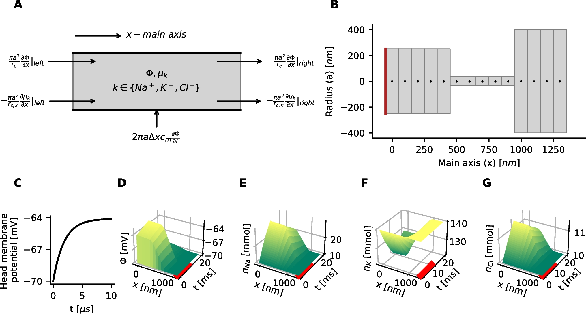
We first study the response of the neuron to a non-fluctuating constant periodic synaptic current. Suppose the target neuron receives constant numbers \(\rho _E\) and \(\rho _I\) of excitatory and inhibitory spikes per unit time, with all the excitatory spikes having the same strength \(w_E\) and all the inhibitory spikes having the strength \(w_I\). The conductance of the excitatory channels \(g_(t)\) is modified by excitatory spikes arriving at times \(s<t\) :

$$\begin g_(t) = \int _^ g_^0 w_E \rho _E exp(-\dfrac^}) ds = g_^0 w_E \rho _E \tau _^ \end$$

(5)

The same formula applies for the constant inhibitory current. The potential of the target neuron fed by this current will reach a stationary value. If this stationary limit is greater than \(V_\) then the target neuron will fire periodically. This constraint reads as :

$$\begin \rho _I < \dfrac*(V_ - V_) + g_^0*w_E*\rho _E*\tau * V_}^0*w_I*\tau (V_ - V_) } \end$$

(6)

The stationary limit of the potential is a weighted average of reverse potentials,

$$\begin V_ = \dfracV_ + g_^0 w_E \rho _E \tau V_ + g_^0 w_I \rho _I \tau V_ } + g_^0 w_E \rho _E \tau + g_^0 w_I \rho _I \tau } \end$$

(7)

If input rates satisfy Eq. 6, the output firing rate will be

$$\begin \rho _ = (g_ + g_^0 w_E \rho _E \tau + g_^0 w_I \rho _I \tau ) * (\log \dfrac - V_} - V_ } )^ \end$$

(8)

The left-dashed curves in Fig. 1 show the output firing rate for three different values of excitatory input rate versus inhibitory input rate. In the rest of this section we take the input to the neuron as stationary homogeneous Poissonian inhibitory and excitatory spike trains. In this case the number of spikes in a time interval \(\Delta t\) follows a Poisson distribution:

$$\begin p(k_) = (\lambda \Delta T)^k \dfrac} \end$$

(9)

The output firing rate of the neuron to the Poisson input is depicted in Fig. 1A. Compared to the constant input with the same constant rate as the Poisson rate \(\lambda\), the curve becomes smoother and the transition from silent state to active state does not show a sharp jump. Below the critical inhibition value, the neuron output follows the mean-field deterministic trajectory, however close to this point the fluctuation effect caused by stochastic arrival of spikes manifests itself. Moreover, the stochasticity in the input leads to stochastic firing at the output. Figure 1B shows how the coefficient of variation of the firing time interval of the output spike train change according to the input. This quantity is calculated as

$$\begin CV(\delta t ) = \dfrac} \end$$

(10)

where \(\delta t\) is the set of firing time intervals of the response of the target neuron subjected to a stationary Poisson input. When the excitatory input is much stronger than the inhibitory one the output firing pattern becomes more regular and the CV value is small. However, close to the inhibition cutoff, CV becomes close to unity, which is characteristic of the Poisson point process.

By using diffusion approximation and Fokker-Planck formalism for the time evolution of membrane potential probability density function, we have derived analytic results for average , variance and CV of inter-spike intervals(ISI) of a neuron receiving subthreshhold average input (see SM Sect. 1.2). We have also calculated the gain function of single neurons in the Gaussian approximation and improve the approximation for the potential distribution and the firing rate by considering the auto correlation in the conductance using the \(\tau\) expansion method to account for first-order corrections to the Fokker-Planck equation. (see SM Sect. 1.1.1)

A Firing rates of a neuron receiving excitatory Poisson input with two different excitatory rates (the red curve corresponding to the higher one) vs. the Poisson inhibitory input. Dashed lines are the response of the neuron to the constant input with a magnitude equal to the Poisson rates (Eq. 8). B Coefficient of variation of the spike intervals of a neuron receiving Poisson inputs of the same rates as in the left graph. Near cutoff, the neuron fires with CV close to one

We end up with the following expression for the CV of the time interval between spikes:

$$\begin CV^2 = \dfrac \approx 1 + \dfrac \mid V_)^2} + 2\sqrtln(2) \dfrac - \langle V \rangle } \sigma }} \mid x_0)^2 } \end$$

(11)

in which,

$$\begin \begin \sigma ^2&= \dfrac\^2 w_E^2 \rho _E( v_ - \langle V \rangle )^2 + \tau ^2 g_^2 w_I^2 \rho _I( v_ - \langle V \rangle )^2 \} \\ b&= \dfrac (g_ + g^0_ w_E \rho _E \tau + g^0_ w_I \rho _I \tau ) \end \end$$

(12)

and C is a negative constant (see Eq. S22 of SM) that monotonically goes to zero as \(x_ := V_ -\langle V \rangle\) increases. In the limit of large \(x_\), the second and the third term both go to zero and CV approaches 1. However, in the near threshold approximation the maximum of the third term in Eq. 11 occurs where CV is approaching 1. Expanding in powers of \(x_\) , we arrive at

$$\begin x_^ := V_ - \langle V \rangle _ = \dfrac} \end$$

(13)

As shown in SM Sect. (1.1.2), \(\dfrac}\) reaches a constant value for high input rates. This can be used to determine the value of \(\langle V \rangle _\) that leads to maximal CV.

Figure 2 shows the CV of the interspike interval for different sets of excitatory and inhibitory pairs of input. As can be seen, at the threshold, neuronal firing time intervals have lower variance, but the CV approaches one far away from the threshold. The stationary membrane potential value corresponding to the maximal value of CV from Eq. 11 is shown in the right diagram and it matches well with the actual values from the simulation. At \(V_:= \langle V \rangle _^ \approx -0.56 mv\), the CV for different input rates has a maximum independently of the rate values.

In the middle plot, we see that the inhibitory rate which satisfies \(CV=CV_\) varies linearly with the excitatory rates. As can be seen, when the stationary membrane potential is approximately below \(V_\), the CV of interspike intervals approaches 1, independently of the values of inhibitory and excitatory rates. This is an indicator that output firing in response to Poisson input is itself a Poisson point process when \(\langle V \rangle _\) lies below \(V_P\) . For a more conclusive result, one has to calculate higher moments or investigate the limit of the FPT probability density when \(x_\) is very large. The fact that the Poisson output condition for different sets of Poisson input leads to approximately a similar level of the membrane potential enables us to introduce the linearization of the output rate at the line corresponding to \(\langle V_\rangle = V_p\).

A CV of interspike intervals for four different excitatory input rates and their corresponding inhibitory rates, which set the average membrane potential at each specified value shown in the x-axis. (Red curve corresponds to the highest excitatory rate (4000Hz) and the blue one to the lowest rate (1000Hz)) B Inhibitory rate vs. excitatory rate at the maximal CV. C Membrane potential value at the value of the maximal CV

Here we want to show that linearizing the response curve of a neuron receiving Poisson current near \(V_P\), introduced in the last subsection, leads to a good approximation for the firing rate of the neuron in a wide range of input rates. The linearization is around the line characterized by Eq. 7 with \(V_= V_\) in the \(\rho _ - \rho _\) plane. This line corresponds to the balance of mean excitation and inhibition at \(V_\). On this balance line, the output rate will depend linearly on the excitatory or inhibitory input rate (see Fig. 3 and E.S21 in SM).

Response of a population of neurons receiving excitatory and inhibitory inputs balanced in a way that the drift term has a fixed point at \(V_P = -0.56mv\). A Output firing rate for different values of balanced inhibitory and excitatory input rates. The output rate changes semi-linearly on this line and firing in this regime that is driven by the fluctuation in the input causes the neuron to fire with Poisson point process statistics. B The stationary potential distribution of the population of neurons. There is a reservoir of neurons close to the threshold while the average firing rate is about 20 Hz. Parameters used: \(w_E\) = 0.5, \(w_I= 0.75\), \(N_E= 7000\), \(N_I=0.25* N_E\)

We want to linearize the output rate around \(V_P\) . For this purpose let us write the equation of the plane passing through the line of current balance at \(V_P\) (Eq. 14) and the tangent line in the \((\rho _E , \rho _ )\) plane at some arbitary point \(( \rho _^0 , \rho _^0 , \rho _^0)\). The balance condition line for an excitatory neuron connected to \(k_\) excitatory neurons and \(k_\) inhibitory neurons each firing with the rate \(\rho _E\) and \(\rho _I\), respectively, and receiving external excitatory rate \(\rho _\) is of the form:

$$\begin \begin \rho _E^e * k_&= \dfrac - V_)*g_^0*w_}^0*w_*(V_- V_)} \rho _I *k_ \\&\quad + \dfrac(V_ - V_) }^0*w_*(V_-V_)} - \dfrac^e}} \end \end$$

(14)

We rewrite this in simpler form as \(\rho _E^e = k \rho _I +C\). The equations for the balance line and the other tangent line in the \((\rho _E , \rho _ )\) plane are

$$\begin \begin&\dfrac = \rho _I - \rho _I^0 = \dfrac - \rho _^0 }} \\&\dfrac} = \rho _E - \rho _E^0 \end \end$$

(15)

Therefore, the equation of the plane passing through these lines is of the form

$$\begin ( \rho _ - \rho _^0 ) =&\beta _ ( \rho _E - \rho _E^0) + ( \alpha _-\beta _k )(\rho _I - \rho _I^0) \end$$

(16)

\(\beta _\) is the derivative of the nonlinear response at the selected point in the direction of \(\rho _E\), and \(\alpha _\) is proportional to the change of output rate by changing inhibition and accordingly excitation on the balance line. These derivatives do not vary much on the balance line, therefore, the choice of the linearization point does not matter for us at this stage. This suggests that the plane of Eq. 16 is tangent to the \(\rho _\) surface. This linear approximation, however, fails for very high excitatory input where the saturation of the neuron causes non-linearity. The linearization point is where the output firing curve has the lowest curvature, and therefore the second derivative vanishes, which makes the approximation error minimal. Figure 4 shows the output firing rate of the target neuron and the linear approximation presented above.

In the next section, we want to investigate the homogeneous firing state of a network. For this purpose we will look at self consistency solutions \(\rho _ = \rho _E(in) = \rho _E^*\) for an arbitrary value of inhibitory current. From Eq. 16 :

$$\begin (1 - \beta _) \rho _E^* = ( \alpha _-\beta _k )(\rho _I - \rho _I^0) + \rho _O^0 - \beta _\rho _E^0 \end$$

(17)

Putting in \(k\rho _I^0 - \rho _E^0 = -C\) and dividing the above equation by \(\beta _\), we arrive at

$$\begin (\dfrac} - 1 ) \rho _E^* = - k\rho _I -C + \dfrac}} (\rho _I - \rho _I^0 ) + \dfrac}\rho _O^0 \end$$

(18)

\(\beta _\) depends on the number of excitatory input to the cell, \(K_\), and is related to the proportional change of output firing at the balance line to the change in the firing rate in each excitatory neuron. On the other hand, \(\alpha _\), proportional to change in the firing rate while fixing the balance condition, is much smaller than \(\beta _\). Therefore, when \(K_\) is large, the self-consistency equation matches the balance line of Eq. 14 with a minimal error.

A Firing rate of a neuron w.r.t. different values of constant inhibitory and excitatory input. B The same for Poisson input. C The linear approximation for the output on the critical line of Eq. 14. D The error of the linear Poisson neuron approximation

As we have seen for sets of Poisson input that produce low firing output the statistics of spiking events resembles a Poisson process. In a population of neurons there might be a stable stationary or oscillatory population rate with Poisson firing of individual neurons. In this case, the magnitude of fluctuations in the population average scales as O(N). This inhomogeneous synchronous or asynchronous firing state exists only in the low firing regime. In the high firing state, the large imbalance of excitatory and inhibitory input leads to periodic firing of the individual neurons which can be also synchronized with high amplitude and high frequency oscillatory population rates. We can use the linear Poisson approximation for identifying and analyzing the dynamics in the low firing rate regime which is of most interest to us. In a homogenous population, solutions of the self-consistency equations for both inhibitory and excitatory neurons’ average output firing rate receiving synaptic currents originated from both neurons in the population and external inhibitory and excitatory currents \(\lambda\) can be written as follows:

$$\begin \rho _^&= f( k_\rho _^ , k_ \rho _^ ,\lambda _ , \lambda _ ) \end$$

(19)

$$\begin \rho _^&= g( k_\rho _^ , k_ \rho _^ ,\lambda _ , \lambda _ ) \end$$

(20)

for \(\rho _ , \rho _ \in [0, \rho _ ]\) . Functions f and g are called excitatory and inhibitory gain functions and \(k_\) is the number of internal connections between neurons in the population. Solving for these gain functions in the general case is not analytically tractable for the EI population. Dynamics to the stationary rates given by Eqs. 19-20 can be phenomenologically approximated by the following mean field equations:

$$\begin \begin \dfrac}&= - \dfrac(\rho _E(t) - f( k_\rho _(t) , k_ \rho _(t) ,\lambda _ , \lambda _ )) \\ \dfrac}&= -\dfrac(\rho _I(t) - g( k_\rho _(t) , k_ \rho _(t) ,\lambda _ , \lambda _ ) ) \end \end$$

(21)

This set of equations may have multiple solutions and changing control parameters can lead to Hopf and saddle-node bifurcations, which in turn produce/destroy oscillations or produce/destroy pairs of fixed points. Although it is possible to numerically investigate the Fokker-Planck equations (FPE) for probability density functions of membrane potentials in the EI population and its bifurcation diagram, in the next subsections, we follow another approach by using linearized nullclines approximation and logistic function approximation for functions f and g. We show that studying these model systems is appropriate for the bifurcation analysis and agrees with simulation results.

Function f in the Eq. 19 for the stationary excitatory rate is of the form of an S-shape or sigmoidal curve. Therefore, this equation has one or three solutions depending on the value of the inhibitory rate. This is shown in Fig. 5A for three different total inhibitory currents. Figure 5D shows the solutions to the Eq. 19 for a typical sigmoidal gain function and different values of total inhibitory current to the excitatory population. This is plotted for two different values of \(w_\) with the dashed curve corresponding to higher \(w_\).

A Excitatory neuron output rate vs. excitatory input rate at three fixed values of inhibitory currents. Increasing Inh. current shifts the gain function to the right. The intersection of the curve and the line \(\rho _E^ = \rho _E^\) are fixed points of the firing rate equation in the homogenous network. B Linearized excitatory gain function. Linearization is performed at the inflection point of the curve and the output firing rate is bounded to the interval \([0,\rho _]\) C Inhibitory neuron output rate vs. inhibitory input at three different values of excitatory current.Increasing Exc. current shifts the gain function to the right. The intersection of the curve and the line \(\rho _I^ = \rho _I^\) are fixed points of the firing rate equation in the homogenous network. D Excitatory nullclines of Eqs. 19-20 for two different values of \(w_\) with the dotted curve corresponding to the higher value. E Linearization of the excitatory nullcline F Inhibitory nullcline and its linearization based on Eqs. 22-23 (dotted curve)

Similarly, Fig. 5C is the plot corresponding to the Eq. 20. Here, the nonlinear sigmoid function g is plotted for three different values of excitatory current. There exists a single intersection between the line passing through the origin and these curves, which means Eq. 20 has a unique solution for the stationary inhibitory rate at each specific excitatory input. Figure 5F is the plot of the location of these intersections for different values of inhibitory input. As can be seen in Fig. 5, there exists a semilinear section in the nullcline graphs corresponding to solutions in the linear Poisson section of gain functions. Based on the linear Poisson approximation of the Sect. 3.1.1, the equations for these lines in both excitatory and inhibitory nullcline graphs are:

$$\begin \begin \rho _E^ * k_&= \dfrac - V_)*g_^0*w_}^0*w_*V_} \rho _I *k_ \\&\quad + \dfrac(V_ - V_) }^0*w_*V_} - \dfrac}} \end \end$$

(22)

$$\begin \begin \rho _E^ * k_&= \dfrac - V_)*g_^0*w_}^0*w_*V_} \rho _I * k_ \\&\quad + \dfrac(V_ - V_) }^0*w_*V_} - \dfrac}} \end \end$$

(23)

where \(k_\) is the number of excitatory/inhibitory synapse to an excitatory/inhibitory neuron. In the remainder of this work, we assume external inhibiotry currents to be zero, in line with our assumption that inhibition is local in our model. We assume \(\dfrac}} = \dfrac}}\), which simplifies our analysis.

In the \(\rho _ - \rho _\) plane the slope and the y-intercept of the two lines in Eqs. 22-23 determine the intersection of the two nonlinear nullclines and can be used to find approximate locations of the bifurcation points of Eq. 21. We choose \(\langle w_\rangle\) and \(\rho _=\lambda _\) as control parameters of our model. Therefore, we first discuss how their change affects the nullclines of Eqs. 19-20. Increasing \(\rho _\) moves the sigmoid graph in Fig. 5A upwards causing the low and middle fixed points to move towards each other. For a sufficiently high value of excitatory rate, these fixed points will disappear by a saddle-node bifurcation. In the excitatory nullcline graph (Fig. 5D) increasing \(\rho _\) shifts the graph to the right. Increasing \(W_\) will both reduce the y-intercept of the excitatory nullcline and the slope of the linear section as shown in Fig. 5D. The nullcline for the inhibitory rate equation stays intact under change of control parameters.

The intersections of the inhibitory and excitatory nullclines are solutions of the set of rate Eqs. 19-20. Based on the number of fixed points and their stability, the system can show bi-stability of quiescent and high firing, oscillatory dynamics, avalanches, high synchronized activity, and quiescent state. Investigating the linearized sections of the graphs can help us identify different regimes of activity. The slope and y-intercept of the linear sections of both nullclines can be compared for this purpose. Based on the Poisson neuron approximation there exists a point in control parameter space where the y-intercept and slope of two nullclines are equal. This point is the solution of the following linear constraints:

$$\begin s_ := \dfrack_}k_} = \dfrack_}k_} := s_ \end$$

(24)

$$\begin y_ := \dfrac}k_} = \dfrac}k_} := y_ \end$$

(25)

where d is a constant equal to \(\dfrac(V_ - V_) }^0*(V_-V_)}\).

Figure 6A shows the case in which \(w_w_ > w_w_\) and the y-intercept of the excitatory nullcline is lower than the inhibitory one. This occurs in the regime of a low to moderate imbalance of excitatory and inhibitory external input and high excitatory synaptic weight. In this case, the quiescent and the high firing fixed point are both stable and separated by a saddle. Increasing external excitatory input, the excitatory nullcline are shifted to the right and the middle saddle and quiescent node disappear by a saddle-node bifurcation and only the high firing synchronous state remains (Fig. 6B). Increasing \(w_\) has the same qualitative effect. However, decreasing external input or \(w_\) drives the system to a quiescent state through different sets of bifurcations depending on the initial state of the system and in general on other parameters of the model. This intermediate transition state involves the appearance of a fixed point in the linear section.

Nullcline diagrams corresponding to regimes of bistability (A), high synchronized firing (B), avalanches (C), and oscillatory dynamics (D). Red curves are excitatory nullclines (Eq. 19) and blue curves are inhibitory nullclines (Eq. 20). Filled and empty circles represent stable and unstable fixed points, respectively. In (A), the linearized nullclines obtained from linear Poisson approximation are drawn and the dependence of their slope and y-intercept on weights is shown. (Eqs. 22-23). In (C), the fixed point on the semilinear section is weakly stable or unstable based on the sign of the eigenvalue of the Jacobian with the absolute value near zero

When \(s_ > s_\) while \(y_ < y_\), there is a fixed point in the linear section as depicted in Fig. 6C. We will discuss the stability of the fixed point on the linear segment in the following sections. By increasing external input, the quiescent fixed point and the low saddle move closer to each other while the fixed point on the linear section ascends to higher rate values. After the saddle-node bifurcation at the low rate, only the fixed point on the linear section survives as shown in Fig. 6D. These two arrangements when the fixed points are close to low firing regimes are important for us because of the avalanche dynamics that appear near this region. The intersection point of the nullclines in the semilinear regime can be approximated by the intersection point of the linearized nullclines which is:

$$\begin \begin \rho _E^c&= \dfrac-V_)(c_\rho _ - c_\lambda _) + g_L(V_L - V_)(c_-c_)}c_-c_c_)} \\ \rho _I^c&= \dfrac-V_)(c_\lambda _-c_\rho _) - g_L(V_L - V_)(c_-c_)}c_-c_c_)} \end \end$$

(26)

where \(c_ = k_ w_ g_(V^R_-V_)\) .

As discussed previously, in the intermediate parameter range, the high fixed point might become unstable through either an Andronov-Hopf or a saddle node bifurcation. Figure 7 shows nullcline graphs and population activity when the high fixed point loses stability by a Hopf bifurcation. Figure 7A shows nullclines population activity of a system that has stable high and quiescent fixed points with a saddle node at low rates. By decreasing \(w_\), \(s_\) approaches \(s_\), while sufficient external input guarantees that \(y_ <y_\) during this parameter change. In this particular setup, the inhibitory nullcline is semi-linear and we may speculate that the high fixed point goes through a Hopf bifurcation when the return point of the excitatory nullcline touches the inhibitory nullcline which takes place at some value \(w^*_ \in [0.55,0.75]\). Decreasing \(w_\) further, the high saddle node descends through a linear segment and gets closer to the lower saddle point (Fig. 7B). The limit cycle becomes unstable by a saddle separatrix loop bifurcation. After saddle-node annihilation of low and high saddles,the system will end up in the quiescent state for low values of \(w_\) (Fig. 7C). Neurons are firing synchronously at a high rates in three different sub-populations in the first case. The high oscillatory activity appears in the second regime where the unstable saddle, which is encircled by a stable limit cycle, lies close to the high activity region. The membrane potential distribution, in this case, has a higher variance, and neurons fire asynchronously.

A1-B1-C1 Nullclines for excitatory and inhibitory neuron populations and their corresponding linear approximations of Eqs. 22-23 obtained from network simulation. Values of parameters are \(w_= [0.75\) (A), 0.55 (B), 0.4 (C)]\(, w_= 2 , w_ =1.5 , w_ = 0.6\). A2-B2-C2 Number of active excitatory neurons (dark blue) and active inhibitory neurons (light blue) in each time slot of (0.1ms) for three different values of \(w_\). A3-B3-C2 The corresponding stationary membrane potential distribution. In the asynchronous state, the distribution has higher variance

In addition to oscillatory activity in the middle range of rates, the EI-population can exhibit non-oscillating asynchronous activity which corresponds to a stable fixed point in the linear regime. Figure 8 is the simulation result of the population rates similar to the setup of the Fig. 7 with higher \(W_\), which, as we will see later, makes the fixed point on the linear section stable.

Simulation results of the network with same parameters as in Fig. 7 except for \(w_ =2.4\). The EI population shows asynchronous firing in the medium range of \(w_\). This suggest that there is a stable fixed point at the intersection of the linear segments of the excitatory and inhibitory nullclines

In this section, we approximate gain functions by logistic functions to analyze bifurcation diagrams and approximate locations of bifurcaion points. For this purpose, we consider the gain functions in the following form:

$$\begin \begin g^x(\rho _ , y_x)&= \dfrac})e^} - z_0, \\ y_x&= g_\tau w_ \rho _ ( V_ - V_) + g_\tau (w_\rho _ + \rho _^x) (V_-V_) \\&\quad +g_(V_-V_), \\ z_0&= \dfrac}(V_-V_)}} \end \end$$

(27)

Here, x stands for either excitatory (E) or inhibitory (I) gain functions, which have the same form but different input arguments. \(\rho _^x\) is the external excitatory input to the population x.

At \(y_x=0\), balanced input sets the membrane potential at the threshold value and the output rate is approximately \(g_ = \dfrac})}\). Dependence of the output rate on inhibitory input, when the balance condition at threshold holds, is represented by the function \(\alpha\). At \(y=0\), the output rate is proportional to the standard deviation in the input and it can be written as function of the inhibitory input rate as (see Fig. 9):

$$\begin g_ = b_0 + b_1 \sqrt} \end$$

(28)

which fixes the function \(\alpha (\rho _)\).

Output rate as a function of input inhibitory rate (blue curve), when the excitatory rate is selected in a way that average membrane potential of the neuron is \(V_\). Neuron is operating near a saddle-node bifurcation point at which \(F(I_) = k\sqrt-I^*}\) (red curve)

At equilibrium, the population rates satisfy:

$$\begin \begin \rho _&= g^I(\rho _ , c_\rho _ + c_\rho _ + d\rho _^I) - z_0 \\ \rho _&= g^E(\rho _ , c_\rho _ + c_\rho _ + d\rho _^E) -z_0 \end \end$$

(29)

where \(c_ = c k_ w_(V_ - V_)\). As before, we take \(w_\) and \(\rho _^E\) as control parameters. Therefore, the solution of the first equation in Eq. 29 is independent of control parameters and gives a curve in the \(\rho _-\rho _\) plane. Taking into account that the inverse of \(g(\rho _ , y)\) is \(g^(\rho _ , z) =\dfrac( \log (\dfrac -z}) + \log (\alpha ))\), the equation for the inhibitory nullcline can be written as :

$$\begin \rho _ =&\dfrac}(\dfrac[\log (\dfrac+z_0)} -(\rho _+z_0)}) + \log (\alpha )] - c_\rho _ - d\rho _^E - g_L ) \end$$

(30)

The term in brackets accounts for non-linearity in low and high values of \(\rho _\). The derivative of this term w.r.t. \(\rho _I\) is \(\dfrac}(\rho _ -\rho _)}\), which is very small in the middle range of \(\rho _\) at values close to \(0.5 \rho _\). This is consistent with the fact that nullclines are approximately linear in the middle range of the rates.

To analyze linear stability of the fixed points, we compute derivatives of the gain function:

$$\begin \begin \dfrac&= kc_ g^x(1-\dfrac}) \\ \dfrac&= kc_ g^x(1-\dfrac}) - \dfrac g^x(1-\dfrac})\dfrac \end \end$$

(31)

Here \(g^x\) stands for \(g^I\) or \(g^E\). One can substitute \(\rho _I + z_0\) and \(\rho _E + z_0\) from Eq. 29 for \(g^I\) and \(g^E\), respectively. Therefore, the Jacobian matrix components at the fixed point are:

$$\begin \begin J_&= -1+c_\rho ^E(1-\dfrac}) \\ J_&= c_\rho ^E(1-\dfrac}) - \dfrac\rho ^E(1-\dfrac})\dfrac \\ J_&= c_\rho ^I(1-\dfrac}) \\ J_&=-1+ c_\rho ^I(1-\dfrac}) - \dfrac\rho ^I(1-\dfrac})\dfrac \end \end$$

(32)

Hopf bifurcation occurs at fixed point solutions at which the trace of the Jacobian vanishes and its determinant is positive. On the other hand, at saddle-node bifurcation occurs at points where the determinant vanishes. We proceed to approximate local bifurcation lines in the parameter space.

The condition on zero trace \(Tr(J) = J_+J_=0\) parameterized by the inhibitory nullcline curve (Eq. 30) determines the value for \(w_\) at which a Hopf bifurcation can occur. Next, we should check the positivity of the determinant to sketch the Hopf bifurcation line in the \(w_-\rho _^E\) plane. A point where both determinant and trace of J are zero, is called a Bogdanov-Takens (BT) bifurcation point. In Sect. (2.1) of SM, we showed that when \(\mid c_c\rho _I (1 - \dfrac}) \mid\) is at a moderate value, i.e. sufficiently greater than one, at the BT point we have:

$$\begin c_^ \approx \dfracc_}} \end$$

(33)

If we take number of connections to satisfy \(\dfrac}} = \dfrac}}\), then \(w_^ = \dfracw_}}\). To sketch the saddle-node bifurcation line we should look at solutions to \(det(J) = 0\). Inserting \(\rho _E(\rho _I)\) from Eq. 30 into det(J) , for each point on the inhibitory nullcline, there exists some \(w_\) for which \(det(J)=0\). The only condition to check is \(w_>0\). Again the condition that the excitatory nullcline intersects the inhibitory one at the fixed point determines \(\rho _\). Along the semi-linear section of the nullcline, the condition \(det(J)=0\) translates into the alignment of the slopes of the linearized nullclines. Therefore, along this section \(w_\) varies very little.

Figure 10A shows Hopf and saddle-Node bifurcation lines with parameters written in the caption. As can be seen, there exist two Bogdanov -Takens bifurcation points at low and high values of external input corresponding to the intersection of nullclines in low and high firing rate regimes.

A Local bifurcation diagram in the control parameter plane \((W_ , \rho _)\). The red curve is the Hopf bifurcation line and the blue curves are saddle-node bifurcation lines. The free parameters of the model are \(\rho _^ =300Hz,W_=1,W_=1.8\) and \(W_=0.6\). B Zoom in on the local bifurcation diagram at low firing rates and the corresponding regimes of phase space with different numbers of fixed points. The dashed line is the condition on the equal slope of linearized nullclines and the semi-dashed the line is the condition on equal y-intercepts. The BT point (black dot) is close to the intersection of these lines. In the labeling of regions (Q) denotes the quiescent state fixed point, (L) is the fixed point at low firing rate, (M