2.1 Firing rate model

The firing rate model simulates the long-term dynamics of the average firing rates of components of a network of neuron populations (Caiola & Holmes, 2019). Generally, changes in the average firing rates of the populations with respect to time can be modeled by the following ordinary differential equation:

$$\begin \mathbf \textbf' = -\textbf + \textbf(\textbf+\textbf) \end$$

(1)

In Eq. (1), \(\textbf\) is a vector that contains the firing rates for each population in the network. \(\mathbf \) is a diagonal matrix, and its diagonal entries contain the time constants for each equation. Traditionally, these time constants are assumed to be approximately equivalent to a population’s time membrane constant (Caiola & Holmes, 2019; Wilson & Cowan, 1973; Holgado et al., 2010; Cowan et al., 2016) and we will make the same assumption here. \(\textbf\) is the activation function, which is the driving force of the neuron and will be discussed later in detail. We use unitless weights to model the strength of inhibitory or excitatory synaptic connections between neuron populations, which are the elements of the matrix \(\textbf\). Finally, \(\textbf\) represents the input from outside the modeled neuronal network. We note that for this study, \(\textbf\) will be set to 0 as we explore the dynamics of the closed thalamocortical system.

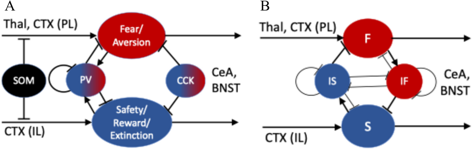
Figure 1 shows the thalamocortical motor circuit (in the grey highlight) and its connection to the basal ganglia (the rightmost grey squares) from a network perspective. We note that this is a simplified model that combines several connections and collaterals between neuron populations. As such, the excitatory thalamocortical connection to corticothalamic layer 5 (CT5) and the inhibitory cortical interneuron connections are represented as one connection and weight (\(w_\)). In addition, the globus pallidus internus (GPi) and substantia nigra pars reticulata (SNr) are combined into one population. Due to the lack of available information on the firing properties of thalamic interneurons, we chose to create two models: denoted the Relay Model and the Full Model.

In the Relay Model, signals from cortical layer 6 (CT6), thalamic reticular neurons (RTNs), and the GPi/SNr are relayed through the IN population and are passed as inhibitory signals to thalamocortical (TC) neurons with no delay. We denote this structure as a relay neuron in Eq. (2). In the Full Model we include the IN population (Eq. (3)). However, due to the lack of IN firing parameters, we arbitrarily chose to use the parameters as for the RTN.

For the Relay Model, we establish the following dynamical system for the average firing rates of the neuron populations in the thalamocortical motor circuit for \(i=1,\dots ,5\):

$$\begin t_iy'_i = -y_i + F_i(\bar_i) \end$$

(2)

with

$$\begin \bar_1&= h \\ \bar_2&= -w_y_1 + w_y_3 + w_y_4- w_y_5 \\&-w_(-w_y_1 - w_y_5 + w_y_4 + b_6) \\ \bar_3&= w_y_2 + w_y_4 \\ \bar_4&= w_y_3 \\ \bar_5&= w_y_4 \\ \end$$

where \(y_1\), \(y_2\), \(y_3\), \(y_4\), and \(y_5\) are respectively the average firing rates of neurons in the GPi/SNr, TC neurons, neurons in CT5, CT6, or RTN.

For the Full Model, we establish a similar dynamical system for \(i=1,\dots ,6\):

$$\begin t_iz'_i = -z_i + F_i(\bar_i) \end$$

(3)

with

$$\begin \bar_1&= h \\ \bar_2&= -v_z_1 + v_z_3 + v_z_4-v_z_5 -v_z_6 \\ \bar_3&= v_z_2 + v_z_4 \\ \bar_4&= v_z_3 \\ \bar_5&= v_z_4 \\ \bar_6&= -v_z_1 + v_z_4-v_z_5 \end$$

where \(z_1\), \(z_2\), \(z_3\), \(z_4\), \(z_5\), and \(z_6\) are respectively the average firing rates of neurons in the GPi, TC neurons, neurons in CT5, CT6, RTN, or IN.

All of these are modeled as functions of time with \(t_i\) as the membrane time constant for the i-th neuron population. \(F_i\) represents the activation function for the i-th neuron population. The positive \(w_\) or \(v_\) denotes the weight that models the synaptic connection from population k to population l with \(w_\) and \(v_\) each representing the difference between the excitatory TC and inhibitory cortical interneuron inputs to CT5 as described above. Although \(w_\) and \(v_\) are differing weights for the Relay Model and Full Model, respectively, they both represent identical synaptic connections in Fig. 1. For simplicity, the models do not consider synaptic and transmission delays and assume that changes in the average firing rates of one neuron population have an instantaneous effect on the others.

2.1.1 Activation function

The “activation function” controls the way by which a neuron discharges in response to stimuli. In our model, the input to the activation function for a certain neuron is the weighted sum of the (momentary) firing rates of all other neurons that are connected to this neuron. Previous studies have suggested that a sigmoidal activation function is usually sufficient to obtain the behavior seen in experiments (Rall, 1955; Wilson & Bevan, 2011; Nambu & Llinas, 1994). However, to allow for an efficient analytical exploration of the impact of different synaptic weights on neuronal firing patterns, we instead used a simpler approach, approximating the sigmoidal activation functions through the use of piece-wise linear (PWL) activation functions of the form (Caiola & Holmes, 2019):

$$\begin F_i(x)= M_i & \text x + b_i \ge M_i\\ x + b_i & \text 0< x + b_i < M_i\\ 0 & \text x + b_i \le 0 \end\right. } \end$$

(4)

where x is the input, \(b_i\) is the baseline firing rate, and \(M_i\) the maximal firing rate.

This activation function restricts a neuron population to fire only above 0 spikes/sec and below its maximum \(M_i\). Within this range, the model neuron responds linearly to inputs. Additionally, if there is no input to the neuron, it fires at its baseline firing rate \(b_i\). Therefore, it properly approximates the major characteristics of a neuron’s sigmoidal firing behavior.

Equation (2) consists of five PWL equations, each with three linear choices, which means that there are in total \(3^5=243\) linear sub-systems to consider and Eq. (3) consists of six PWL equations and \(3^6=729\) linear sub-systems. Because the inputs to the activation functions (i.e., the weighted firing rates) determine which piece is taken, we can divide the phase space (the space of all possible values of firing rates) into 243 regions for the Relay Model and 729 regions for the Full Model, each corresponding to a distinct linear sub-system that can be solved exactly.

Suppose the initial network state starts in region k in the phase space, then the firing rates will change according to the governing equation of region k, until they either stabilize inside this region or undergo changes that place them outside this region. In the latter scenario, the firing rates will then follow the governing equation of the new region. Thus, the originally nonlinear equation now consists of a sequence of linear equations that can be solved analytically.

Furthermore, the firing rate of a neuron should not stabilize at 0 spikes/sec or its maximum. Thus, a physiologically realistic steady state can only be achieved in the model when all activation functions take their middle piece. In the phase space, the unique region that corresponds to this case is further denoted as the middle region.

2.1.2 Solution and stability of the subsystems

Using the PWL activation function, system Eq. (2) can be written for \(i = 1,\dots ,5\) as:

$$\begin t_iy'_i = -y_i + M_i & \text \bar_i + b_1 \ge M_i \\ \bar_i + b_i & \text 0 \le \bar_i +b_1 \le M_i\\ 0 & \text \bar_i +b_1 \le 0 \\ \end\right. } \end$$

(5)

And system Eq. (3) can be written for \(i = 1,\dots ,6\) as:

$$\begin t_iz'_i = -z_i + M_i & \text \bar_i + b_i \ge M_i \\ \bar_i + b_i & \text 0 \le \bar_i + b_i \le M_i\\ 0 & \text \bar_i + b_i \le 0 \\ \end\right. } \end$$

(6)

where each branch in the PWL defines a region in phase space. Identified exact solutions for each region can be combined to create continuous solutions for the entire system. Without loss of generality, a solution in a given region k, can be found by solving the following linear ordinary differential equation,

$$\begin \varvecy'_k(t) = \textbf_k y_k(t) + \textbf_k \end$$

(7)

where \(\varvec\), a diagonal matrix with diagonal entries of \(t_i\), contains membrane time constants, and matrix \(\textbf_k\) and vector \(\textbf_k\) are, respectively, the corresponding coefficients and constant terms for the linear system of region k.

To determine under which conditions the subsystem for region k yields a stable solution, we analyzed the eigenvalues of the matrix \(\textbf_k =\varvec^ \textbf_k\). If region k is stable, all eigenvalues of \(\textbf_k\) will be negative.

2.2 Numerical algorithm

To solve Eqs. (5) and (6), a computational solver based on the method proposed by Caiola and Holmes (2019) was designed. The solver arrives at an exact solution for each linear subsystem and combines the solutions for individual subsystems to obtain the global solution. This, in turn, can be used to determine whether a steady state has been reached (based on the extent of variations of y over time), and whether the firing rate trajectory forms a limit cycle. The latter is said to have occurred if the solution loops back to its initial point within a (negligible) distance of \(10^\). Additionally, the solver was used to visualize solutions by graphing firing rates over time, and to calculate the period of a limit cycle if it exists.

2.3 Parameter justification

For work with Eq. (5), the values of the baseline (\(b_i\)) and maximal firing rates (\(M_i\)) and the membrane time constants (\(t_i\)) for each neuron population were extracted from previous literature. The synaptic weights (\(w_\), \(v_\)) were found by data-fitting algorithms which are described in the next section.

The neuron population modeled in the network fires at its baseline firing rate when it receives no external input. The membrane time constant is the time it takes for a neuron’s firing potential to decay from its resting value to 63% of this resting value after a small hyperpolarizing current application, applied during ex vivo patch clamp experiments (Isokawa, 1997). We used membrane time constants as a surrogate for firing rate constants, following common established practice (Caiola & Holmes, 2019; Holgado et al., 2010; Pavlides et al., 2012, 2015). When possible, the network parameters were sourced from published primate studies on the specific network areas modeled here. When necessary due to a lack of data availability, additional information from other areas of the brain, nearby neurons, or other species (mice, rats, or cats) was also used (Table 1). When multiple sources were found, a conservative blend was used.

Table 1 Intrinsic constant parameters used in the model

Note that there is no information on the baseline firing rate of interneurons in the primate ventral motor thalamus. Data from comparable brain regions in humans and cats (Ison et al., 2011; Putrino et al., 2011) came to differing estimates in interneuronal baseline activity. Given this uncertainty, we arbitrarily chose a baseline value of 22.7 Hz for the thalamic interneurons. In tests with a lower baseline (6 Hz), we noted no substantial changes to system stability (not shown).

2.4 Data fitting2.4.1 In vivo primate neuronal firing rate data

A dataset of primate neuronal firing rates was obtained from in vivo electrophysiological recordings as reported in the literature (Table 2). Given that there is no available data documenting the average spontaneous firing rate in the reticular nucleus in the parkinsonian state, the same firing rate values were used for both healthy and parkinsonian states (Saga et al., 2017). As stated earlier, in the Relay Model the thalamic interneurons are treated as relay neurons, whereas in the Full Model the thalamic interneurons use the same parameters as the RTN: none of the IN firing rates are not based on experimental observations.

Table 2 Firing rate estimates used in data fitting2.4.2 Error function

The initial goal of this work was to find a set of synaptic weights for which the average firing rates simulated by the model would fit the experimental data for each of the two scenarios: (1) a “healthy” model, and (2) a “parkinsonian” model. To achieve this goal, an error function was implemented in MATLAB, with subsequent optimization to minimize the squared differences between the model simulated firing rates and the data. The optimization aimed to minimize the squared error between model-predicted steady-state (healthy) or cycle-averaged (parkinsonian) firing rates and experimental data. For the parkinsonian state, an additional penalty term, \(E_f\) was included. This term penalized simulated oscillation frequencies falling outside the physiologically relevant beta band (\(13-30\) Hz), thereby ensuring that emergent oscillatory activity occurred within the correct frequency range, while the primary fitting target remained the average firing rates.

\(H_i\) was defined as the experimental healthy state average firing rate of a neuron population i, with a standard deviation of \(H_i^\sigma \), and \(\bar\) was defined as the firing rate output of the corresponding population in the model. The difference between experimental and model simulated data was weighted by the associated standard deviation to penalize errors outside one standard deviation of the experiment data. Therefore, an error function was constructed as a weighted sum of squared differences as follows:

$$\begin E_H = \sum _^ \left( \frac}}\right) ^2 \end$$

(8)

For the model of the parkinsonian state, \(P_i\) was defined as the experimental firing rate, with its associated standard deviation \(P_i^\sigma \). Since firing rates in the parkinsonian state may oscillate, the model output \(\bar\) was taken as the average firing rate of neuron population i over one cycle of oscillation. Therefore, the error function is

$$\begin E_P = \sum _^ \left( \frac}}\right) ^ \end$$

(9)

As mentioned earlier, we forced the simulated frequency of oscillations, f, to fall into the beta-band (\(13-30\) Hz), by adding \(E_f\) to penalize oscillation greater than 30 Hz or smaller than 13 Hz as such:

$$\begin&E_P' = \sum _^ \left( \frac}}\right) ^2 + E_f(f) \\ \text \;\;\;\;&E_f(f) = \nonumber (f-30)^2 & \text f>30 \\ 0 & \text 13 \le f \le 30 \\ (f-13)^2 & \text f<13 \\ \end\right. } \end$$

(10)

2.4.3 Coupled weight search

Given a set of synaptic weights with which the model was matched to healthy firing rate data, we investigated whether the model could be matched to firing rate data recorded in the parkinsonian state by changing only a small number of the weights. This effort required fitting the model to both the healthy and the parkinsonian data simultaneously, using two sets of slightly differing weights. We called this process the “coupled weight search”, as the two sets of weights obtained are closely related to each other. The coupled weight search answers the question of whether it is possible for the system to bifurcate from a healthy to a parkinsonian state with changes in a few specific connections.

In the coupled weight search, the error function was taken to be the sum of the firing rate errors for both healthy and parkinsonian states, including the penalty for firing rate oscillations outside of the beta-band, to minimize the overall error for the coupled solutions. Using the notations from the previous section, the error function was defined as \(E = E_H + E_P + E_f\).

2.4.4 Constrained optimization

MATLAB’s genetic algorithm (GA) was used to search for weights that can minimize the errors. The GA solver’s input is an error function, an initial guess, lower and upper bounds, and a function that describes the constraints on the parameters. GA randomly generates a set of weights at each iteration and selects the ones that are best at minimizing the error function. This technique allows the GA to search a wide range of weight space with less probability of getting caught in a local minimum as can occur with other optimization solvers.