1 Introduction

Advancements in diffusion magnetic resonance imaging (dMRI) have facilitated our understanding of the brain's intricate architecture and organization (Le Bihan, 2003). By measuring the diffusion of water molecules within the brain tissue, dMRI provides valuable information to investigate the connectivity and assess the white matter (WM) microstructure of pathways in the brain. Voxels in the WM can contain different axonal fiber populations with complex configurations (Jeurissen et al., 2013). Each one of these populations is called fixel, which denotes the discrete component of a fiber element (Raffelt et al., 2015; Tournier et al., 2019). Fixels and their properties, like orientation and tissue metrics, are fully determined by the voxel in which they reside. Local modeling allows for estimating these fixel properties at each voxel of the dMRI data (Alexander et al., 2017; Jelescu and Budde, 2017). Tractography can use these locally estimated fixel orientations to reconstructs the trajectories of the WM, which are often called streamlines (Behrens et al., 2007; Jeurissen et al., 2017). Additionally, tractometry (Jones et al., 2005; Yeatman et al., 2012) has emerged as a useful method for quantitative analysis of the WM pathways. It encompasses the streamlines obtained with tractography at the macroscopic level with the metrics obtained from a local modeling method at the microscopic level. This combination enables the analysis of microstructural changes by extracting quantitative metrics along specific WM anatomical tracts. Tractometry insights could potentially serve as a valuable tool for investigating WM characterization and degeneration associated with neurological disorders, such as multiple sclerosis (MS) (Winter et al., 2021; Beaudoin et al., 2021), Alzheimer's disease (Lee et al., 2015), and traumatic brain injury (Huang et al., 2022), among others.

Diffusion Tensor Imaging (DTI) (Basser et al., 1994) is a single fiber method traditionally used to estimate properties of the fixels, averaging the diffusion properties of all the fixels within a voxel. Thus, DTI results in a loss of important information of the fixels, especially when different fiber populations with different properties or lesions are present within the same voxel. This presents an important problem in estimation because WM tissue contains between 66% to 90% of voxels with crossing fibers (Descoteaux, 2008; Jeurissen et al., 2013; Schilling et al., 2017). DTI Limitations motivated the development of more advanced acquisition and local modeling techniques. Multi-shell High Angular Resolution Diffusion Imaging (HARDI) (Tuch et al., 2002) was originally developed to provide anisotropy measures beyond DTI metrics (Tournier et al., 2011) that are more robust to crossing fibers and sensitive to WM alterations, making also tractography more robust (Descoteaux, 2015). HARDI allowed to develop techniques that estimate multiple fixels within a voxel. Notable examples of these techniques are: Q-ball Imaging (QBI) (Tuch, 2004; Descoteaux et al., 2007), the Multi-Tensor Model (MTM) (Tuch et al., 2002), and Constrained Spherical Deconvolution (CSD) (Tournier et al., 2007). In particular, MTM is a straightforward extension of DTI that represents each one of the fiber populations in the voxel by a different diffusion tensor. However, the estimation of MTM parameters is an ill-posed challenging problem, that requires very high SNR data and large computational resources, restricting it's routine clinical use.

The dMRI signal arising from the WM is composed of several compartments. Thus, taking advantage of HARDI, several techniques were developed to decompose the dMRI data into contributions from various compartments. An example of these multi-compartment methods procedures is the model in Novikov et al. (2019), which depicts the dMRI data as a combination of Intra-Cellular (IC), Extra-Cellular (EC) and ISOtropic (ISO) contributions. Other hybrid methods are based in the MTM like the Free-Water DTI (FW-DTI) (Pasternak et al., 2009), which fits for each voxel a bi-tensor model including an anisotropic tensor for tissue compartment and an isotropic tensor for a free water compartment. The DIstribution of Anisotropic MicrO-structural eNvironments with Diffusion-weighted imaging (DIAMOND) (Scherrer et al., 2015) and the Multi-Resolution Discrete-Search (MRDS) (Coronado-Leija et al., 2017) are more general MTM-based methods, which fits up to three restricted anisotropic tensors for the restricted and hindered diffusion compartments and one isotropic tensor for the free diffusion compartment.

DTI (Basser et al., 1994) metrics are the most widely used metrics for tractometry (Jones et al., 2005). Although DTI metrics have the potential to be biomarkers, they have inconsistent sensitivity to characterize the WM as they are easily biased. For example, the common Fractional Anisotropy (FA) metric is informative about changes in WM microstructure caused by pathology, but crossing fibers bias it. FA decreases in fiber crossing voxels because oblate tensors are obtained, which leads to an alteration in the resulting FA tract profile in the tractometry as shown in Figure 1. These alterations can be confused with alterations derived from WM degeneration, which is also illustrated in Figure 1, leading to erroneous or ambiguous interpretations. Moreover, in the presence of crossing fibers together with pathology, FA increases, which could seem counterintuitive. However, this could happen, when only one of the fiber populations in the crossing is affected by the pathology, then the resulting single-tensor may become sharper, see Figure 2. Approaches that have studied other DTI metrics, like the radial diffusivity (RD) metric, have shown that RD is a promising biomarker for demyelination (Song et al., 2002, 2005; de Vries, 2010). However, they have reported that RD can be inconsistent, presenting challenges in its reliability and reproducibility and resulting in misleading results. Besides, co-existing inflammation, edema, and crossing fibers can significantly impact on the DTI metrics at the same time (Ye et al., 2020).

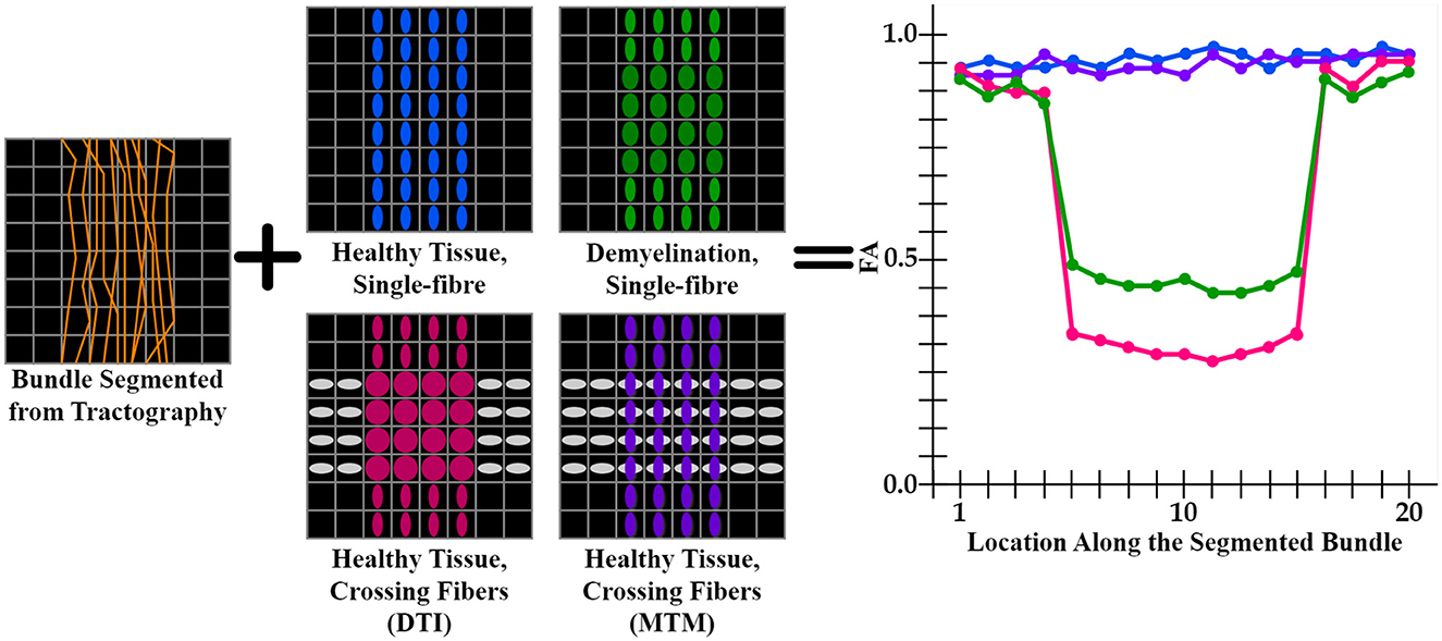
Figure 1. Illustration of an FA tract profile in 4 different scenarios showing the limitation of DTI-based tractometry. All FA tract profiles are generated through the same bundle (orange streamlines). Blue, green, pink tensor fields exhibit a single fixel in each voxel estimated with DTI, while purple tensor field exhibits a multi-fixel estimation with MTM. (blue tensors) A control case with healthy tissue and only one fiber population. This scenario is expected to have high FA values in the tract profile (blue curve). (green tensors) A single fiber with demyelination resulted in an increased RD and decreased FA (green curve). (gray and pink tensors) Tensors are estimated using DTI, where FA is affected in the intersection as oblate tensors are obtained (pink curve). (gray and purple tensors) Tensors are estimated using MTM, which can estimate a different tensor for each fixel at the intersection. This case is expected to have normal FA values as the tractometry only considers FA values of the tensors aligned with the streamlines (purple curve). From this scheme, it is clear that a single-fixel analysis is limited when differentiating between demyelination and crossing fibers based only on the alterations in the tract profiles.

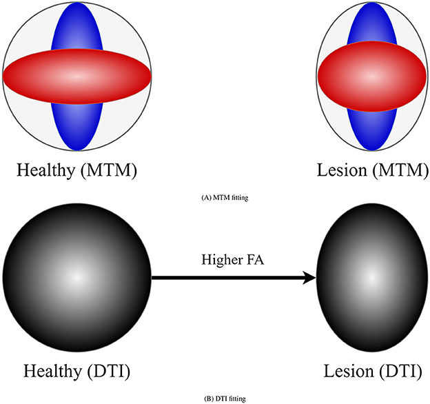
Figure 2. Example of how DTI can lead to counter-intuitive results in the presence of a lesion and crossing fibers. (A) Represents a MTM fitting showing the presence of crossing fibers in two scenarios: healthy (left) and damaged (right) tissue. Left scenario exhibits two healthy fiber populations. Right scenario shows a healthy fiber population and another with lesion. (B) Represents a tensor obtained with DTI in the healthy and damaged scenarios. In the presence of lesion DTI shows a sharper tensor, leading to a higher FA compared with the healthy scenario. This is a consequence of a lesion only in one of the underlying fiber populations for which DTI is not sensitive.

Multi-fixel methods have further expanded the scope of tractometry, resulting in tract-specific analyses less impacted by crossing fibers. Remarkable examples are the Automated Fiber-tract Quantification (Yeatman et al., 2012; Kruper et al., 2021), the Connectivity-based Fixel Enhancement (Raffelt et al., 2015), the Fixel-Based Analysis framework (Dhollander et al., 2021), the Tractometry_flow pipeline (Cousineau et al., 2017; Kurtzer et al., 2017; Di Tommaso et al., 2017) and, recently, the UNRAVEL framework (Delinte et al., 2023). Other tractometry frameworks have combined DTI metrics with other metrics including fixel-based metrics like the Apparent Fiber Density (AFD). For example, the framework called Profilometry (Dayan et al., 2015) performs a simultaneous analysis of DTI metrics and other metrics, resulting in tract profiles as parameterized curves in a multi-dimensional space. Nonetheless, the crossing fibers bias in DTI metrics still limits it. Besides, these types of multi-fixel methods face several challenges and limitations. As example, frameworks informed with CSD metrics such as AFD, while sensitive, do not have a straightforward biological interpretation; moreover, they could be biased as CSD employ a fixed response function across the entire WM (Dell'Acqua et al., 2007; Jones et al., 2013). On the other hand, previous tractometry results using MTM fixel-based metrics are not free of limitations. For instance, they need more complex multi-shell dMRI acquisitions (Scherrer and Warfield, 2012) and are limited to a maximum of 2 fixels per voxel (Delinte et al., 2023). This is insufficient in many brain regions, e.g. the centrum semiovale, where 3 fiber populations cross from the corticospinal tract, corpus callosum, and superior longitudinal tract intersect. Additionally, fixel-FA estimation has shown to be affected by high levels of noise and inconsistent through scan-rescan experiments (Mishra et al., 2014) as a consequence of MTM fitting being numerically unstable (Tuch et al., 2002). MTM-based methods generally struggle to accurately estimate the required number of tensors per voxel (N). These methods tend to overestimate the value of N as a direct consequence that a single diffusion tensor does not properly represent the dMRI signal (even when a single fixel is present) for b-values higher than 1ms/μm2, needing more tensors to fit the per voxel signal (Karaman et al., 2023).

Between the MTM-based methods, MRDS offers a balanced trade-off in terms of model complexity and accuracy when using short-acquisition-time clinical multi-shell dMRI data (Coronado-Leija et al., 2017). MRDS has proven to be a noise-robust and accurate multi-fixel method for estimating the directions of the fixels and their metrics. In addition, MRDS has been histologically validated in a rat model of unilateral retinal ischemia in which only one of the optic nerves was damaged. This nerve lesion was correctly detected by MRDS at the region where the optic nerves cross (optic chiasm) (Rojas-Vite et al., 2019). Moreover, MRDS has shown to be capable of recognizing 3 fiber populations in regions-of-interest (ROI) like the centrum semioval (Hernandez-Gutierrez et al., 2021) when using clinical in vivo multi-shell dMRI data. A recent work (Karaman et al., 2023) has proposed to use the Track Orientation Density Imaging (TODI) (Dhollander et al., 2014) as a useful spatial regularizer for a more accurate and robust estimation of N in MRDS. The Track Orientation Distribution (TOD) image estimated with TODI presents an increased amount of spatial consistency compared with the fiber orientation distribution (FOD) image obtained with constrained spherical deconvolution (CSD) (Dhollander et al., 2014).

In this paper, we propose a novel tractometry pipeline to address several current limitations of tractometry informed with multi-fixed methods. Our proposed pipeline combines multi-tensor fixel-based metrics estimated with MRDS and the Tractoflow (Theaud et al., 2020) and Tractometry_flow (Cousineau et al., 2017; Kurtzer et al., 2017; Di Tommaso et al., 2017) pipelines. The proposed pipeline provides fixel-based tensor metrics that are robust to crossing fibers and noise. Provided fixel-based metrics have the potential to be biomarkers for pathologies like demyelination and can be useful for the characterization and study of underlying WM anomalies in patients with pathologies such as MS. Most of the previous tractometry studies in pathology used DTI metrics, then, our multi-tensor pipeline results can be straightforwardly situated in their context and compared with them. Finally, the pipeline is tested on both synthetic phantom dMRI data and clinical dMRI in vivo data from a large healthy control and MS groups with a scan-rescan experiment, highlighting the robustness and potential of our approach when studying WM anomalies in patients with such neurological disorders.

2 Methods

In this section, we describe the simulation of the synthetic phantom and the acquired in-vivo dMRI data. We also explain each step in the proposed pipeline.

2.1 Synthetic data

A synthetic phantom was generated based on the geometry of a previously published dMRI phantom (Caruyer et al., 2014), see Figure 3. The size of the phantom is 50 × 50 × 50 voxels with an isotropic dimension of 1.0mm. Similar to Caruyer et al. (2014), our synthetic phantom has 20 distinct bundles showing a complex fiber crossing configuration and volume contamination with CerebroSpinal Fluid (CSF). Each bundle in the phantom exhibits unique diffusivities and axonal dispersion characteristics. The diffusivities of each bundle were tuned to mimic those found in healthy human brains (Coelho et al., 2022).

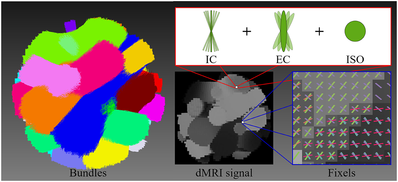
Figure 3. This figure illustrates the geometry of the diffusion MRI (dMRI) phantom, the multi-compartment model employed for signal generation, and the resulting signal. The geometric structure of the phantom is composed of 20 bundles, highlighting each bundle with a different color. The multi-compartment model (intracellular, extracellular, and free water compartments) that is used to generate the shown dMRI signal at each voxel includes axonal dispersion. The figure illustrates the orientations of fixels, depicting the crossing fiber configuration and distribution.

We have simulated a phantom dMRI signal for each individual bundle and the whole volume signal without noise and without dispersion. Then, DTI was fitted to each individual bundle signal as well as the whole dMRI signal, and the tensor metrics were extracted. This simulated dataset was employed as Gold Standard (GS) to compare results with the experiments on in-vivo dMRI data. A multi-compartment model also known as Standard Model (SM) (Ferizi et al., 2016; Novikov et al., 2019), was adopted to simulate this phantom signal by including three types of microstructural environments: intracellular (IC), extracellular (EC), and isotropic (ISO). Each environment was simulated with a given volume fraction denoted by fic, fec and fiso, respectively. The IC space was modeled with cylinders of zero radius (sticks), the EC space with a cylindrically symmetric tensor (zeppelin), and finally, the ISO space was modeled as a free diffusion compartment (ball) (Panagiotaki et al., 2012; Ferizi et al., 2013a,b).

Three datasets were generated with known GS. The radial EC diffusivities were simulated based on Fieremans et al. (2012). Thus, the EC space tortuosity D0/Dec⊥, which quantifies how the diffusion is affected by cellular and extracellular structures within tissue, was defined as the ratio of free diffusivity D0=2μm2/ms over the EC diffusivity Dec⊥. Therefore, the intracellular volume fraction fic was most sensitive to axonal loss. Besides, it was most sensitive to demyelination. The first dataset incorporated Dic∥ and Dec∥ diffusivities within a healthy range sampling a Gaussian distribution with a mean of 2μm2/ms and variance of 0.01μm2/ms, while Dec⊥=0.48μm2/ms, fic = 0.65 and fec = 1−fic. On the other hand, the second dataset simulated, in some bundles, conditions associated with demyelination on MS. Specifically, in regions with demyelination fic = 0.55 and Dec⊥=0.71μm2/ms, while in regions without damage, the values remained the same as in the first dataset. Finally, our third dataset simulated conditions related to axonal loss. For this case, fic = 0.35 and Dec⊥=0.59μm2/ms in regions with lesion and regions without lesion maintained the same control values as the first dataset. All datasets were generated with a high and realistic noise level (SNR = 12). The isotropic diffusivity Diso and volume fraction fiso were fixed equal to 3μm2/ms and 0.05, respectively. Axonal dispersion was modeled with a Watson distribution (Jespersen et al., 2012, 2018). The κ value of each bundle used as the parameter for the Watson distribution was sampled from a Gaussian distribution with mean 20 and variance 0.01. Lastly, we used the same protocol of the in-vivo data described below.

The 13th bundle of the phantom was selected to compare the three scenarios above because bundle 13 crosses with 2 and 3 bundles at different places. In the datasets simulating damages, the lesion was simulated in a spot of the bundle represented by the red region, while the diffusivities outside the lesion remained the same as in the control case.

2.2 In-vivo data

Two groups of participants were recruited from the University of Sherbrooke (UdS) and the Center Hospitalier Universitaire of Sherbrooke (CHUS) community. The first group was a healthy control (HC) group with 26 adults, and the second group has 22 relapsing-remitting MS patients. Both groups had a gender proportion of 75% women and 25% men. Diffusion MRI data was acquired using a clinical 3T MRI scanner (Ingenia, Philips Healthcare) using a 32-channel head coil. Each subject was scanned 5 times over 6 months and a 4-week interval (±1 week) with a total acquisition time of 20 minutes for each session. MRI acquisitions were obtained for each subject at roughly the same time daily to mitigate potential diurnal impacts, i.e. morning subjects underwent all sessions in the morning with a permissible 2-3-hour variation. Finally, 6 of the 26 healthy control subjects were discarded for several reasons, including problems during the scan or processing. Thus, the HC group employed for the experiments had 20 subjects.

All MRI images were aligned respect to the anterior commissure-posterior commissure plane (AC-PC), which is an anatomical reference defined by two small bundles in the brain. One bundle located in the front part of the brain, and the other in the back. This ensured consistency in the orientation and position of the images when analyzing them across scans and subjects. In addition, 3 type of data were included:

• Anatomical 3D T1-weighted image (T1): an MPRAGE image was acquired axially at 1.0mm isotropic resolution.

• Multi-shell diffusion-weighted images (DWI): these images were acquired with a single-shot EPI spin-echo sequence at 2.0mm isotropic resolution. The acquisition scheme included 100 unique gradient directions uniformly distributed over and across 3 shells at b-values b = 0.3ms/μm2 (8 directions), b = 1ms/μm2 (32 directions) and b = 2ms/μm2 (60 directions) with 7 non-diffusion-weighted images (b = 0) for a total of 107 diffusion volumes. An additional reversed phase-encoded b = 0 image was acquired after the DWI acquisition with the same geometry to correct EPI distortions.

• Inhomogeneous magnetization transfer images (ihMT): these images were acquired using a 3D segmented-EPI gradient-echo sequence with different magnetization transfer (MT) preparation pulses. They have 2 × 2 mm resolution and 65 slices with 2.0 mm thickness.

Finally, all images have been subjected to visual quality assessment. A detailed and more extensive data description can be found in Edde et al. (2023).

2.3 Pipeline

The data processing pipeline consists of 6 key steps described in sequential order in the following subsections, see Figure 4:

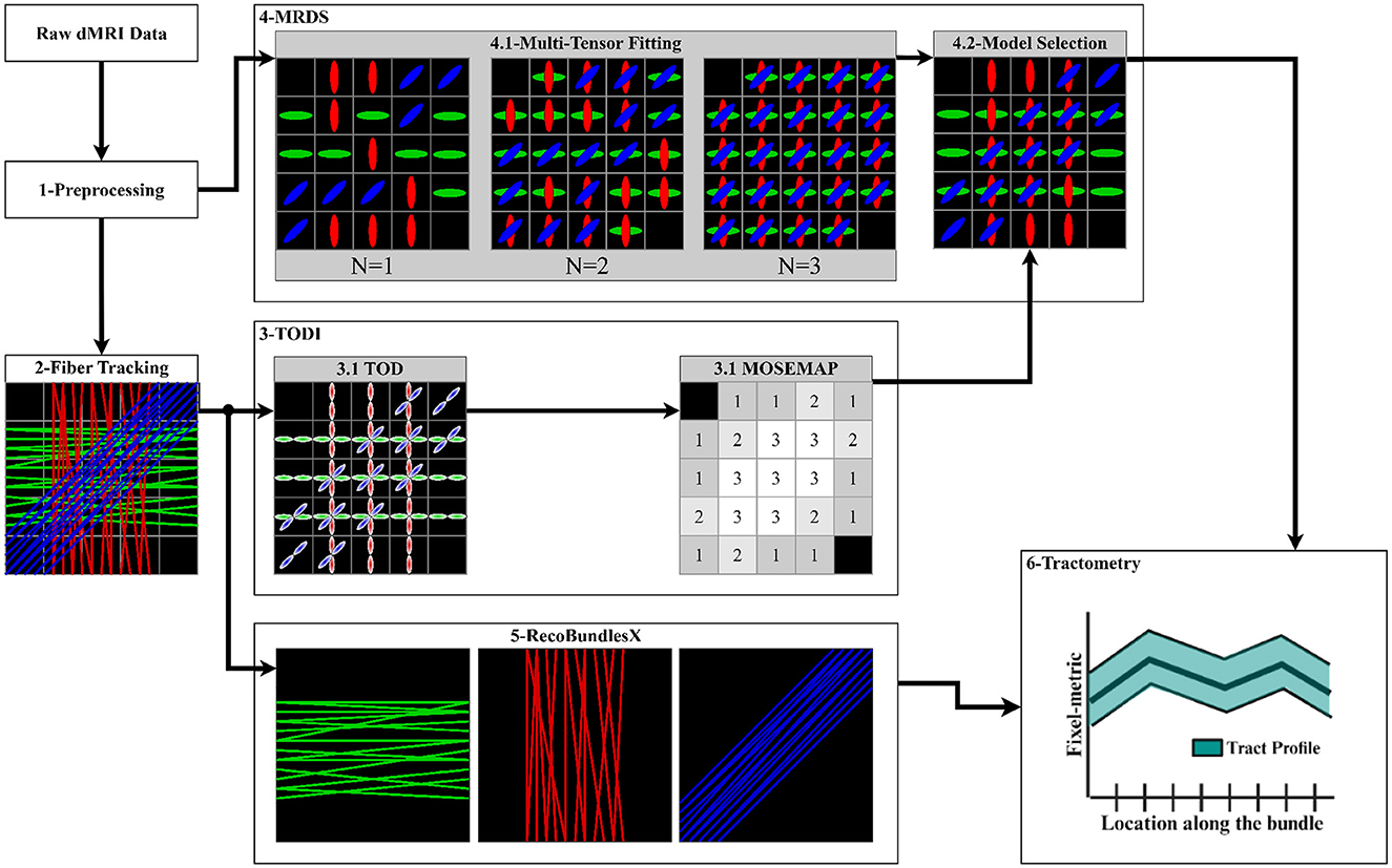
Figure 4. Proposed pipeline to extract the tract profiles using the MRDS fixel-based multi-tensor metrics. (1) Input data is denoised, aligned, corrected, normalized, cropped, and resampled. Brain, WM, and lesion masks are extracted. (2) The CSD method is fitted to obtain an FOD image, and a local tracking technique is used to estimate the streamlines. The WM mask is used to seed the streamlines. (3) TODI maps the tractogram into a NuFO map, which MRDS exploits as a model selection map in the MTM fitting. (4.1) MTM is fitted to the dMRI data using MRDS. MTM parameters are estimated for N = 1, N = 2, and N = 3, resulting in 3 MTFs. (4.2) The TODI NuFO map is used on the estimated MTFs to choose a value of N that better describes the diffusion signal at each voxel. TODI helps to refine the MTF with the spatial information provided by the tractogram (Karaman et al., 2023). Multi-tensor fixel-based metrics are computed from the MTF derived from the model selection. (5) The tractogram is segmented into major fiber bundles using the RecoBundlesX pipeline. (6) Segmented bundles and estimated fixel-metrics are the input of the Tractometry_flow pipeline to assess a tract profile for every combination of the bundles and metrics.

2.3.1 Preprocessing

The preprocessing of the dMRI data was performed using the Tractoflow pipeline (Theaud et al., 2020). This includes the brain and WM masks extraction, T1 registration and tractography.

The dMRI data was denoised using the MP-PCA (Veraart et al., 2016) method. Brain deformation induced by magnetic field susceptibility artifacts was corrected (Andersson et al., 2003). Motion artifacts corrections and slice-wise outlier detection were performed (Andersson and Sotiropoulos, 2016). Image intensities were normalized to reduce the bias by the magnetic field (Tustison et al., 2010). The brain mask was obtained from the bet command from FSL (Smith, 2002). Specifically, Tractoflow performed an extraction on the b = 0 image. Then, the obtained mask was applied to the whole DWI to remove the skull and prepare the DWI for the T1 Registration. Tractoflow performed brain extraction after Eddy/Topup correction to have a distortion-free brain mask.

Tractoflow processed the T1 image using eight different steps. First, Tractoflow preprocessed the T1 image including denoising, correcting and resampling steps for the T1 image. Then, the T1 image was registered on the b = 0 and FA images using the nonlinear SyN ANTs (antsRegistration) multivariate option, where the T1 image is set as moving image and the b0 and FA images are set as target images. After registration, Tractoflow extracted gray matter (GM), white matter (WM) and cerebrospinal fluid (CSF) partial volume masks using fast from FSL. These maps were used to compute the exclusion and inclusion maps for tractography (Girard et al., 2014), which are anatomical constraints for the tracking (Smith et al., 2012; Girard et al., 2014).

2.3.2 Fiber tracking

The fiber tracking was also done using the Tractoflow pipeline. The seeding mask employed in the tractography was the obtained WM mask. The tractogram was generated employing the anatomically constrained particle filter tracking (PFT) algorithm (Girard et al., 2014). This algorithm utilized the FOD image obtained with the Multi-Shell Multi-Tissue Constrained Spherical Deconvolution (MSMT-CSD) (Jeurissen et al., 2014), along with the inclusion map, exclusion map, and a seeding mask to guide the tractography process. The seeding mask employed in the tractography was the extracted WM mask. A fully detailed explanation of the whole Tractoflow pipeline can be found in Theaud et al. (2020).

Additionally, Tractoflow includes strategies to avoid premature track termination when tracking MS patients. The seeding mask in MS patients was filled using a lesion-corrected WM mask. During the tracking process, if a peak in the FOD image is coherent and well-defined, the tracking continues even if the voxel is inside a WM lesion, increasing anatomical accuracy and consistency in obtained tractograms for MS patients. This step can be omitted as the tractogram can be generated with any fiber tracking technique.

2.3.3 TODI as model selector

The tractogram from fiber tracking was then processed with the TODI method to obtain a TOD image. Subsequently, the resulting TOD image was segmented to produce discrete fixels (Smith et al., 2013). Then, the fixel-based image was converted into a Number of Fiber Orientations (NuFO) scalar image, where the number of fixels was counted in each voxel. A threshold peak amplitude was utilized to prune the spurious peaks, such that any lobe for which the maximal peak amplitude was smaller than 0.1 was omitted. Finally, this NuFO image was used as input MOSEMAP in MRDS, which is better described in the next step (Section 2.3.4).

2.3.4 Multi-tensor Fitting

The MTM represents the diffusion signal Si at each voxel as:

Si/S0=∑j=1Nαjexp(-bigiTDjgi),i=1,…M,    (1)

where M is the number of unitary gradient orientations gi, N is the number of tensors, and αj is the fraction of the j-th diffusion tensor Dj. Assuming axial symmetry, then Dj is parameterized by the unitary principal diffusion direction (PDD) θj, the axial (λj∥) and radial (λj⊥) diffusivities, such that:

giTDjgi=λj∥(θj·gi)2+λj⊥[1-(θj·gi)2]    (2)

The bundle-specific parameters of the MTM were non-linearly estimated using the MRDS (Coronado-Leija et al., 2017) method for N = 1, N = 2, and N = 3, resulting in 3 multi-tensor fields (MTFs), see Figure 4. More than three fixels can be estimated, albeit with increased computation time and reduced precision for the estimated parameters. Besides, N ≤ 3 has been reported to be a reasonable threshold (Jeurissen et al., 2013). Initial diffusivities for the non-linear estimation of parameters in Equation 2 were obtained from DTI at brain WM voxels with a high probability of containing only one fiber.

Given that high b-value diffusion signals are not fully represented with the diffusion tensor, causing an overestimation in N. Thus, the original statistical model selection in MRDS, which provides a model selection map (MOSEMAP) with the value of N that better describes the diffusion signal at each voxel, is replaced for the NuFO scalar map obtained with TODI in step 2.3.3. The TODI NuFO scalar map merges the 3 MTFs into a reevaluated and refined MTF with the spatially smoothed information provided by the tractogram (Karaman et al., 2023), see Figure 4. From this improved MTF, fixel-FA, fixel-MD, fixel-AD, and fixel-RD maps were generated. The fixel-FA map maintains the same spatial dimensions as the original DWI Each voxel may contain multiple tensors. Then, an extra layer was added to store the multiple fixel-FA values obtained at each voxel. The scalar fixel-FA value was obtained for every tensor within a voxel, computed as the standard FA (Basser et al., 1994). This resulted in a 4D-dimensional fixel-FA map. The computation of fixel-RD, fixel-AD and fixel-MD maps was analogous to the computation of the fixel-FA map. Similarly, a map storing the PPDs of the MTF was computed. These maps were used as input for the tractometry step.

2.3.5 Tractogram segmentation

The tractogram was segmented into major bundles employing the RecoBundlesX (St-Onge et al., 2023, 2020; Kurtzer et al., 2017; Di Tommaso et al., 2017) pipeline, see Figure 4. RecoBundlesX recognizes bundles by comparing the subject's tractogram with a template (or atlas) through a similarity metric based on their shapes. This algorithm is re-evaluated multiple times with parameter variations and label fusion because RecoBundlesX is a multi-atlas and multi-parameter approach. We used the atlas in Rheault (2023), which is designed specifically to be used with RecoBundlesX, and it was built from delineation informed with anatomical priors (Catani and Thiebaut de Schotten, 2008). After RecoBundlesX identified a large number of WM bundles, tracks were visually inspected to ensure their quality. The Superior Longitudinal Fasciculus (SLF), Arcuate Fasciculus (AF), Pyramidal Tract (PYT), Inferior Longitudinal Fasciculus (ILF), Inferior Fronto-Occipital Fasciculus (IFOF), Middle Cerebellar Peduncle (MCP) and Cingulum (CG) bundles were selected to showcase the pipeline's capabilities. Selected bundles comprise a large set covering most of the brain, showing complex crossing fiber configurations, which is why they are frequently studied in the literature (Yeatman et al., 2012; Mishra et al., 2014; Chamberland et al., 2019; Winter et al., 2021).

In the experiments with MS patients, we have chosen the AF, ILF, IFOF and PYT bundles, which have clinical implications in the context of MS studies (Filippi and Rocca, 2011). The AF bundle connects the frontal and temporal lobes, crucial in speech communication. On the other hand, the ILF bundle connects the occipital and temporal lobes. Its functionality includes visual processing, tracking and recognition of objects and obstacles. Like AF and ILF, the IFOF bundle is involved in speech communication and visual processing tasks, transporting signals from the frontal to occipital and temporal lobes. The PYT connects the spinal cord with the cerebral cortex. It is essential in voluntary control movements. Therefore, when MS lesions appear in the AF, ILF, IFOF, and PYT bundles, several symptoms are experienced by MS patients. These symptoms include difficulties in speech and comprehension, visual deterioration, visual memory problems, attention issues, and affected motor coordination.

2.3.6 Tractometry with fixel-based metrics

The proposed pipeline employed the Tractometry_flow (Cousineau et al., 2017; Kurtzer et al., 2017; Di Tommaso et al., 2017) pipeline, which delivers metric maps along each individual input bundle. Then, each metric map was projected through every bundle to obtain a tract profile. We adapted the Tractometry_flow pipeline to support multi-tensor fixel-based metrics. The closest-fixel-only (Raffelt et al., 2015) strategy was used to map the contribution of the multi-fixels estimated by MRDS to a given streamline.

2.4 Experiments

We designed three experiments to study the behavior of the pipeline:

• Experiment I: our proposed pipeline is tested on the three synthetic phantom datasets described before, simulating healthy tissue, demyelination and axonal degeneration. Estimated multi-tensor fixel-based metrics and tractometry results are compared with the known GS of the phantom. Relative errors obtained using the formula error=|valuereal-valueestimated|valuereal are reported in the results.

• Experiment II: the pipeline is used to study the robustness to crossing fibers of the tract profiles in the in-vivo healthy control group. Obtained tract profiles informed with multi-tensor fixel-based metrics of the 100 total scans (20 subjects scanned 5 times each one) are group-averaged and compared to DTI-derived tract profiles.

• Experiment III: the pipeline is employed to study variations of metrics across the AF, ILF, IFOF and PYT, which are relevant bundles in the study of relapsing-remitting MS. As the location and severity of the MS lesions are different for every individual patient, it is irrelevant to make a group-averaged study of the MS group of patients. Instead, we have manually selected patients 004 and 022 because they have the most severe and larger white matter coverage of lesions present in the WM. These particular patients are chosen in an effort to maximize the difference between the healthy control group and the MS patient tract profiles. Individual patient tract profiles informed with multi-tensor fixel-based metrics are compared with the group-averaged tract profiles in order to exhibit differences.

3 Results 3.1 Experiments on synthetic data

In Figure 5, we show violin plots comparing single-tensor (blue) and multi-tensor (green) metrics. Horizontal lines refer to the GS (red) and the mean of each distribution. Single-tensor metrics exhibit several discrepancies with respect to the GS, most DTI distributions are bimodal, such that one of the peaks is close to the GS, while the other is underestimated for FA and AD, and overestimated for RD.

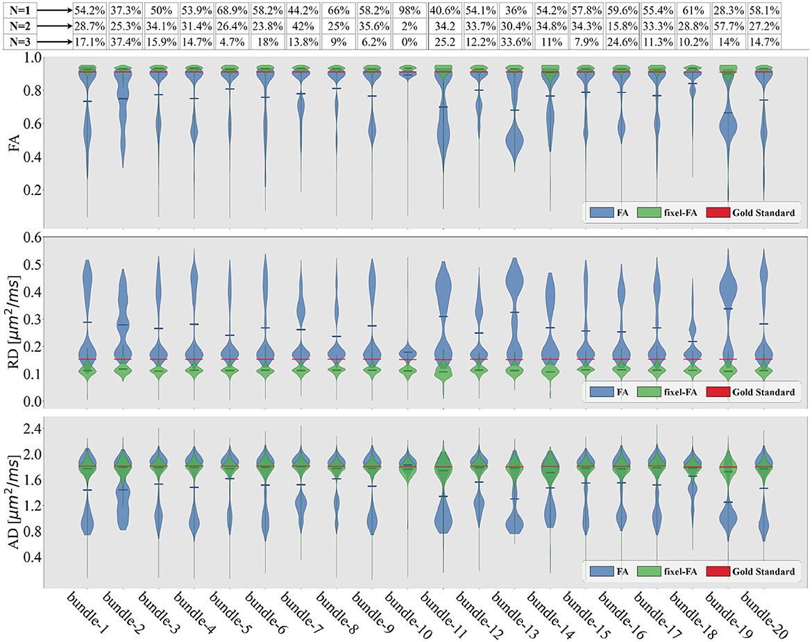
Figure 5. Violin plots of the estimated tensor and multi-tensor fixel-based metric maps along each bundle of the control synthetic dataset (control values without lesions). Tensor metrics are estimated with DTI (blue violin) and multi-tensor fixel-based metrics with MRDS (green violins). Obtained metrics are compared with the GS (red line). The bundle's average crossing fibers composition in the GS is indicated in the proportions containing N = 1 fiber, N = 2, or N = 3 fibers at the top of the figure.

For each bundle, we accounted for the proportion of voxels containing 1, 2, and 3 fiber populations using the NuFO map obtained with TODI, i.e., we accounted for the proportions of N. These proportions are at the top of Figure 5. By inspecting percentages of N shown in Figure 5, it is reasonable to assume that DTI bimodality is caused by crossing fiber biases. In Figure 5, bundles with a high proportion of N = 2 and N = 3 have a more pronounced bimodality; this is particularly evident for the 13th bundle. In contrast, it can be seen in Figure 5 that the mean of the estimated fixel-FA and fixel-AD are similar to the GS value in all bundles. The relative error of fixel-FA and fixel-AD is around 10% as it is reported in Table 1, reaching a relative error as low as 2.7% in some bundles where the average relative error is 5.6%. It is important to note that, for fixel-based metrics, the relative error of bundles with a high count of 2 and 3 crossing fibers is similar to the relative error in bundles exposing mostly single fiber composition. As an example, percentages shown in Figure 5 exhibit that bundles 5 and 10 mainly have no crossing fibers, while bundle 11 has, for the most part, crossing fibers. However, the relative error of fixel-FA for bundles 5, 10, and 11 in Table 1 are around 3%. Even for the bundle 13, which is one of the most challenging bundle as it has a high proportion of crossing fibers, the relative error remains at 7%. Values in Table 1 exhibit a higher relative error for fixel-RD compared with fixel-AD and fixel-FA, but still less relative error than RD in general. Additionally, bundle 2 shows abnormal relative errors compared to the other bundles.

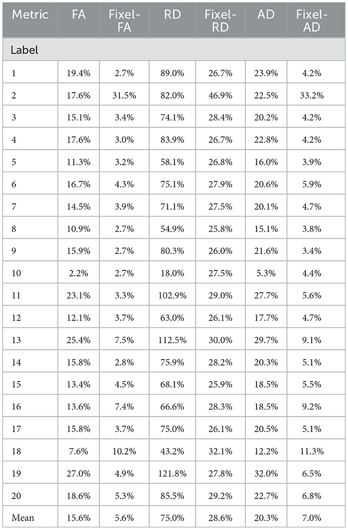
Table 1. Relative errors of the violin plots for the tensor (blue) and multi-tensor (green) metric maps estimated with DTI and MRDS, respectively.

Looking at the obtained tractogram, the streamline count for bundle number 2 after segmentation is 104, which is insufficient to cover the whole bundle's volume, resulting in an increased relative error. Thus, results in bundle 2 should be interpreted with caution because of the low number of streamlines. Bundle 10 has almost 100% single fiber composition. It is the only bundle where the relative error of RD is less than the one reported in fixel-RD. This suggests that, in the absence of crossing fibers, DTI's RD may be more accurate than fixel-RD. Besides, fixel-RD violin plots in Figure 5 indicate that, in general, fixel-RD tends to underestimate the GS value, which is congruent with the relative errors reported in Table 1. In the MTM fitting with MRDS the isotropic volume fraction is overestimated, see Appendix A. Since the synthetic data was generated using a multi-compartment model and MTM does not fully represent the signal for the b-values in our protocol, then the ISO compartment may be partially explaining the contribution of the EC compartment (see Appendix A for more details). Therefore, this underestimation of the fixel-RD metric might be related to the overestimation of the isotropic volume fraction.

Similar to Figure 5, in Figure 6 violin plots on the 13th bundle are reported for the 3 simulated scenarios detailed in Section 2.1: healthy control case, demyelination, and axonal loss. Additionally, tractometry results on the same bundle for the 3 different scenarios can be found in Figure 6B. In the healthy control scenario, the limitations of DTI in capturing the overall WM microstructure configuration are evident. Tract profiles informed with standard DTI metrics are biased by crossing fibers as FA, RD, and AD tract profiles have variations along the bundle, while the GS does not. In particular, FA tract profile decreases and RD tract profile increases when the value of N increases, see Figure 6B. In contrast, the robustness of the multi-tensor fixel-based metrics estimated with MRDS is evident as they provide tract profiles independent of the underlying fiber configuration, see Figure 6B.

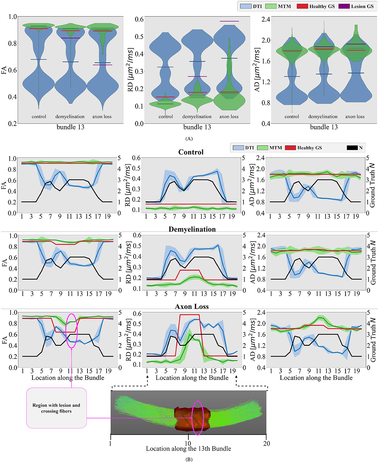
Figure 6. Differences between different simulated scenarios are studied in the bundle number 13 of the phantom. (A) Violin plots of the estimated single-tensor (blue) and multi-tensor (green) fixel-based metrics for each scenario. The mean of the distributions is represented as a horizontal line matching the color of the distribution. The GS of the healthy tissue and damaged tissue are represented as red and purple horizontal lines, respectively. (B) Tract profiles resulting from projecting the estimated single- and multi-tensor fixel-based metrics along the 13th bundle. Every row represents a different scenario (control, demyelination, and axon loss), while every row represents a different measure (FA, RD, and AD). The GS value of N (black curve) and tensor metrics (red curve) are also projected on the bundle number 13, showing the actual underlying fiber configuration along this bundle for comparison. A region with lesions and crossing fibers is highlighted in pink.

In the demyelination scenario, results with DTI metrics in Figure 6 showed limited sensitivity to changes in the WM microstructure. In the region with a lesion, tract profiles exhibit variations, but they do not correspond with the GS. Contrarily, results with multi-tensor fixel-based metrics show enhanced sensitivity, detecting reductions in FA and increase in RD associated with simulated demyelination while maintaining robustness to noise and crossing fibers, see Figure 6. Like the demyelination scenario, DTI metrics exhibit limitations in detecting axonal loss, particularly in regions with crossing fibers. Despite the differences in the three simulated scenarios, results in Figure 6 show no substantial differences in DTI metrics. This makes it impossible to distinguish between different scenarios. Results with multi-tensor fixel-based metrics are less contaminated by fiber crossing artifacts, which allows to detect variations in the tract profiles related to lesions. Obtained tract profiles informed with fixel-based metrics underestimate the GS RD, which is expected and congruent with the results investigated in Figure 5. Although results with multi-tensor fixel-based metrics overestimate the GS FA and underestimate the GS RD, they are accurate in shape and sensitive to small variations.

3.2 Experiments on in-vivo data

For experiments on in-vivo data, we focus only on FA and RD metrics and their fixel-based counterparts, as MS research and literature report that FA and RD are potential biomarkers closely related to microstructure anomalies and demyelination (Song et al., 2002, 2005). Figure 7 illustrates tract profiles for different major bundles in the left hemisphere of the healthy participants.

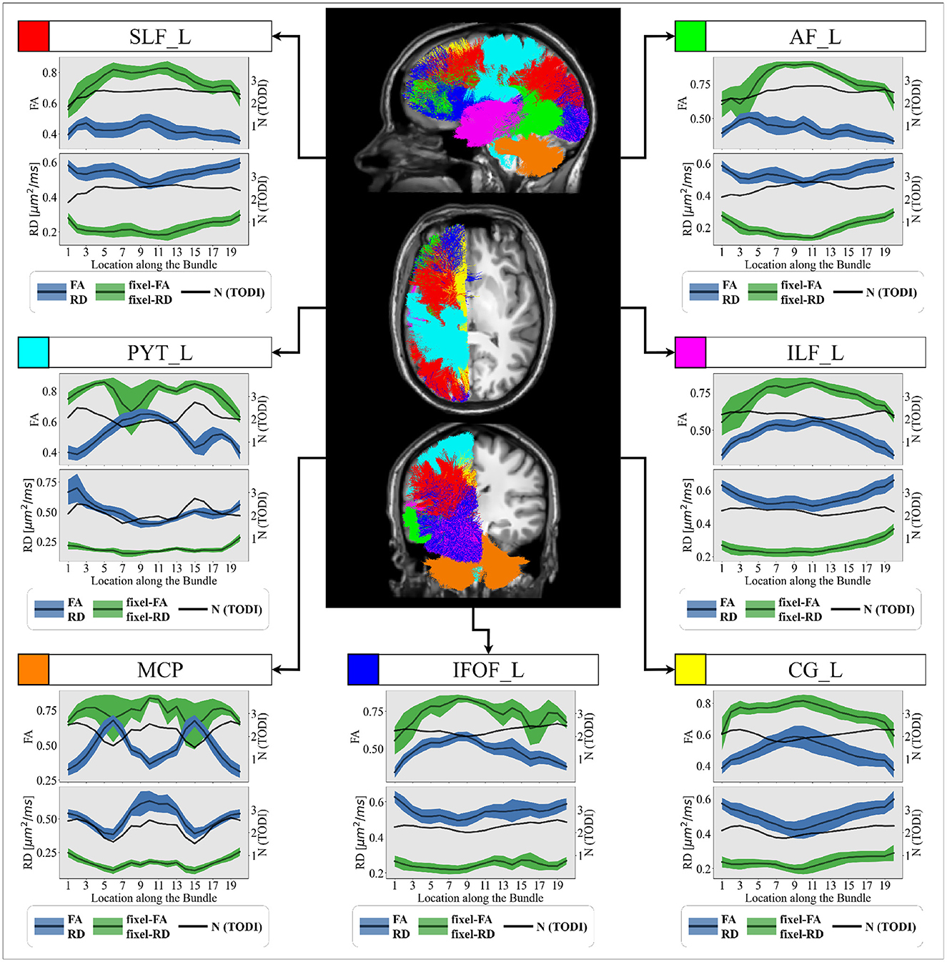
Figure 7. Group-averaged tract profiles of the 100 healthy control scans (comprising 20 participants scanned five times over 6 months) along several segmented WM bundles: the (red) SLF_L, (cyan) PYT_L, (orange) MCP, (blue) IFOF_L, (yellow) CG_L (magenta) ILF_L and (green) AF_L bundles. The mean and variance of the trac