Introduction

Emotion recognition (Jia et al., 2021; Tan et al., 2020; Cimtay et al., 2020; Doma and Pirouz, 2020) has become an important task in affective computing. It has potential applications in areas like affective brain-computer interfaces, diagnosing affective disorders, detecting emotions in patients with consciousness disorders, emotion detection of drivers, mental workload estimation, and cognitive neuroscience. Emotion is a mental and physiological state that arises from various sensory and cognitive inputs, significantly influencing human behavior in daily life (Jia et al., 2021). Emotion is a response to both internal and external stimuli. Physiological signals, such as Electrocardiography (ECG), Electromyography (EMG), and Electroencephalography (EEG), correspond to the physiological responses caused by emotions. They are more reliable indicators of emotional expression than non-physiological signals, such as speech, posture, and facial expression, which can be masked by humans (Tan et al., 2020; Cimtay et al., 2020). Among these physiological signals, EEG signals have a high temporal resolution and a wealth of information, which can reveal subtle changes in emotions, making them more suitable for emotion recognition than other physiological signals (Atkinson and Campos, 2016). EEG-based emotion recognition methods are more accurate and objective, as some studies have verified the relationship between EEG signals and emotions (Xing et al., 2019).

In recent years, EEG signals have gained widespread application in emotion recognition due to their ability to accurately reflect the genuine emotions of subjects (Jia et al., 2020; Zhou et al., 2023). Early approaches to EEG-based emotion recognition have relied on processes such as signal denoising, feature design, and classifier learning. For example, Wang et al. have introduced the Support Vector Machine (SVM) classifier (Wang et al., 2011), while Bahari et al. have proposed the K-Nearest Neighbors (KNN) classifier (Bahari and Janghorbani, 2013), both achieving effective emotion classification. However, traditional machine learning techniques have been constrained by intricate feature engineering and selection processes. To overcome these limitations, researchers have introduced deep learning techniques. The continuous refinement of deep learning algorithms has led to significant achievements in EEG-based emotion recognition. For example, Kwon et al. have utilized CNN to extract features from EEG signals, while Li et al. have obtained deep representations of all EEG electrode signals using Recurrent Neural Networks (RNN; Kwon et al., 2018; Li et al., 2020). Additionally, some researchers have adopted hybrid models combining Convolutional Neural Networks (CNN) and RNN. For instance, Ramzan et al. have proposed a parallel CNN and LSTM-RNN deep learning model for emotion recognition and classification (Ramzan and Dawn, 2023). Although traditional neural network models such as CNN and RNN have achieved high accuracy in EEG emotion recognition tasks, they typically process data in the form of grid data. However, grid data cannot effectively represent connections between different brain regions, thus hindering models from directly capturing the spatial topological features of EEG signals. To better capture connections between brain regions and achieve improved performance in emotion recognition tasks, researchers have begun exploring the use of graph data to represent interactions between brain regions and employing Graph Neural Networks (GNNs) to process this data. For instance, Asadzadeh et al. have proposed an emotion recognition method based on EEG source signals using a Graph Neural Network approach (Asadzadeh et al., 2023). However, models based on GNNs face challenges in accurately detecting local features and capturing the spatial activity features of EEG signals.

However, when applying deep learning models to interdisciplinary tasks such as EEG-based emotion recognition, significant challenges arise due to the limited number of subjects in EEG emotion datasets, coupled with individual differences among subjects. This often results in a notable decrease in the performance of deep learning models in cross-subject EEG emotion recognition tasks. To address the issue of poor performance of subjects in EEG emotion recognition, many researchers have begun exploring the application of transfer learning techniques. In cross-subject EEG emotion recognition tasks, transfer learning primarily addresses the issue of domain gaps caused by individual differences. Transfer learning mainly includes fine-tuning and domain adaptation. Fine-tuning, as an effective knowledge transfer method, has gained widespread adoption. Zhang et al. introduced the Self-Training Maximum Classifier Difference (SMCD) model, utilizing fine-tuning to apply a model trained on the source domain to the target domain (Zhang et al., 2023). However, collecting a large amount of labeled data from the target domain requires considerable time, manpower, and financial resources. Especially in tasks like EEG emotion recognition, acquiring large-scale EEG datasets and labeling them is a complex and expensive task. In some cases, labeled data from the target domain may be extremely scarce, or even insufficient for fine-tuning, which limits the performance and generalization ability of the model on the target task. Researchers have begun exploring the application of domain adaptation in cross-disciplinary EEG emotion recognition. Li et al. proposed a Domain Adaptation method that enhances adaptability by minimizing source domain error and aligning latent representations (Li et al., 2019). However, the majority of existing domain adaptation methods only focus on extracting shallow-level features, without effectively aligning deep-level features of different types. This greatly limits the ability of the model for cross-domain transfer learning.

The primary contributions of this paper can be outlined as follows:

• To accurately capture the activity states of different brain regions and their inter-regional connectivity, we have designed a dual-branch Spatial Activity Topological Feature Extractor Module, named SATFEM. This module has been able to simultaneously extract spatial activity features and spatial topological features from EEG signals, significantly enhancing the recognition performance of the model.

• To minimize the disparity between the source and target domains, we have devised a Domain-adaptation Spatial-feature Perception-network for cross-subject EEG emotion recognition, resulting in the proposal of the DSP-EmotionNet model. This model is tailored to enhance the generalization of the model on the target domain, thereby elevating the accuracy of cross-subject EEG emotion recognition tasks.

• The proposed DSP-EmotionNet model achieves accuracy rates of 82.5% and 65.9% on the SEED and SEED-IV datasets, respectively, for cross-subject EEG emotion recognition tasks. These rates surpass those of state-of-the-art models. Additionally, a series of ablation experiments have been conducted to investigate the contributions of key components within DSP-EmotionNet to the recognition performance of cross-subject EEG emotion recognition tasks.

1 Related work

Traditional EEG feature extractors, such as CNNs and RNNs, have limitations in capturing the connections between brain regions, which constrains their ability to extract spatial topological features. Although GNN models have made improvements in this area, they still face challenges in detecting subtle local variations. Domain adaptation techniques have shown success in cross-subject EEG emotion recognition tasks, but most existing domain adaptation-based methods focus predominantly on aligning shallow features, failing to effectively utilize deeper and more diverse feature types.

1.1 EEG spatial activity feature extractor

In recent years, the application of EEG signals in the field of emotion recognition has significantly increased. This is mainly attributed to the accurate and authentic reflection of the true emotional states of individuals by EEG signals. With the development of deep learning, two popular deep learning models, CNN and RNN, have been widely applied in EEG emotion recognition. For instance, Kwon et al. have utilized CNN for feature extraction from EEG signals. In their model, the EEG signal undergoes preprocessing via wavelet transform before convolution, considering both the time and frequency aspects of the EEG signal (Kwon et al., 2018). Li et al. have employed four directed RNNs based on two spatial directions to traverse the electrode signals of two different brain regions, obtaining a deep representation of all EEG electrode signals while preserving their inherent spatial dependencies (Li et al., 2020). Moreover, some researchers have adopted hybrid models combining CNN and RNN. For example, Chakravarthi et al. have proposed a classification method that combines CNN and LSTM, aiming to recognize and classify different emotional states by analyzing EEG data (Chakravarthi et al., 2022). Ramzan et al. have proposed a parallel CNN and Long Short-Term Memory Recurrent Neural Network (LSTM-RNN) deep learning model, which primarily utilizes CNN for extracting spatial features of EEG signals and LSTM-RNN for extracting temporal features of EEG signals, thus achieving emotion recognition and classification (Ramzan and Dawn, 2023). However, EEG spatial activity feature extractors such as CNNs and RNNs typically process data in a grid format. While grid data can effectively reflect the spatial activity states of EEG signals, it fails to adequately represent the connections between different brain regions. This limitation hinders the model's ability to directly capture the spatial topological features of EEG signals.

1.2 EEG spatial topological feature extractor

Despite the high accuracy achieved by traditional neural network models such as CNN and RNN in EEG emotion recognition tasks, the data they handle is typically in the form of grid data. EEG data are usually captured from multiple electrodes on the scalp, with each electrode signal representing the activity of the corresponding brain region. However, grid data cannot effectively represent the connectivity between brain regions, thereby preventing the model from directly capturing the connections between different brain regions. Therefore, in order to better capture the connectivity between brain regions and achieve better performance in emotion recognition tasks, researchers have begun to explore the use of graph data to represent the connections between brain regions and leverage GNNs to process such graph data. For instance, Asadzadeh et al. have proposed an emotion recognition method based on EEG source signals using a Graph Neural Network node (ESB-G3N). This method treats EEG source signals as node signals in graph data, the relationships between EEG source signals as the adjacency matrix of the graph data and employs GNN for EEG emotion recognition (Asadzadeh et al., 2023). However, GNN-based models have certain advantages as EEG spatial topological feature extractors in processing the spatial topological features of EEG signals, they face challenges in accurately detecting local features and subtle variations in brain activity.

1.3 Transfer learning for emotion recognition

Due to the potential applications of deep learning models in various fields, there is great interest in utilizing these models for EEG-based emotion recognition. However, when applying deep learning models to cross-subject EEG emotion recognition tasks, there is a significant challenge due to the limited number of subjects in EEG emotion datasets, coupled with individual differences between subjects. This often results in a significant drop in the performance of deep learning models in interdisciplinary EEG emotion recognition tasks. To address the issue of decreased performance of subjects in EEG emotion recognition, many researchers have begun to explore the application of transfer learning techniques. In interdisciplinary EEG emotion recognition tasks, transfer learning primarily addresses the problem of data domain gaps caused by individual differences. EEG signals from different subjects in the same emotional state may exhibit significant variations due to individual differences. In such cases, the target domain has represented the feature space of EEG data obtained from a certain number of subjects. In contrast, the source domain has included data collected from one or more different individuals. Li et al. have incorporated fine-tuning into emotion recognition networks and examined the extent to which the models can be shared among subjects (Li et al., 2018). Wang et al. have proposed a method that utilizes fine-tuning to address the challenge of emotional differences across different datasets in deep model transfer learning, to construct a robust emotion recognition model (Wang et al., 2020). These methods overcome subject differences by training on the source domain and fine-tuning on the target domain. Although existing transfer learning methods for EEG emotion recognition can achieve improved results, almost all existing work requires the use of a certain amount of labeled data from the target domain for fine-tuning training. However, collecting a large amount of labeled data from the target domain requires a considerable amount of time, manpower, and financial resources. Especially in tasks such as EEG emotion recognition, obtaining large-scale EEG datasets and labeling them is a complex and expensive task. In some cases, the labeled data from the target domain may be extremely scarce or even insufficient for fine-tuning, which may limit the performance and generalization ability of the model on the target task. Therefore, some researchers have begun exploring the application of domain adaptation for cross-subject eeg emotion recognition. For example, Jin et al. have proposed the utilization of the Domain Adaptation Network (DAN) for knowledge transfer in EEG-based emotion recognition to address the fundamental problem of mitigating differences between the source subject and target subject in order to eliminate subject variability (Jin et al., 2017). Li et al. have proposed a domain adaptation method for EEG emotion recognition, which is optimized by minimizing the classification error on the source domain while simultaneously aligning the latent representations of the source and target domains to make them more similar (Li et al., 2019). Wang et al. have proposed an efficient few-label domain adaptation method based on the multi-subject learning model for cross-subject emotion classification tasks with limited EEG data (Wang et al., 2021). However, most existing domain adaptation-based methods for cross-subject EEG emotion recognition focus primarily on aligning shallow features, without effectively aligning and fully utilizing deeper, more diverse types of features.

2 Methodology 2.1 Overview

The overall architecture of the proposed model is illustrated in Figure 1. We summarize three key ideas of the proposed DSP-EmotionNet model as follows: (1) Constructing EEG spatial activity features and EEG spatial topological features. (2) Integrating spatial activity feature extractor and spatial topological feature extractor to capture the connections between different brain regions and the subtle changes in brain activity, this module is named the SATFEM module. The SATFEM module enhances the generalization ability of the model in cross-subject EEG emotion recognition by extracting both spatial activation and spatial topological features, resulting in a more robust feature representation. Compared to traditional methods that focus on a single type of feature, this combined approach better captures the complexity of EEG data. (3) Utilizing the SATFEM module as a feature extractor, a domain adaptation spatial feature perception network was proposed for cross-subject EEG emotion recognition tasks, improving the generalization ability of the model. This method not only applies domain adaptation techniques but also employs a dual-branch feature extractor to ensure effective domain feature alignment between different subjects. This enables domain adaptation to go beyond merely aligning shallow features, allowing for the effective alignment of deeper and more diverse feature types.

Figure 1. The overall architecture of DSP-EmotionNet for EEG emotion recognition is as follows. Initially, two distinct feature maps of the brain are constructed: one representing EEG spatial activity features and the other representing EEG spatial topological features. Subsequently, the spatial activity feature extractor is employed to detect subtle changes in brain activity, and the spatial topological feature extractor is used to capture the connectivity between different brain regions. Finally, a domain adaptation spatial feature perception network is proposed for cross-subject EEG emotion recognition tasks, aimed at enhancing the generalization capability of the model.

2.2 EEG feature representations

In this section, we introduce two distinct EEG feature representations: EEG spatial activity feature representation and EEG spatial topological feature representation. These different feature representations reflect various spatial relationships within the brain. Specifically, We employ EEG spatial activity feature representation to illustrate spatial activation state distribution maps of the brain, which can reflect the activation states of different brain regions in space. We use EEG spatial topological feature representation to depict spatial topological functional connectivity maps of the brain, which can reflect the connectivity between different brain regions in space. These two EEG feature representations complement each other and effectively demonstrate the spatial relationships of EEG signals.

2.2.1 EEG spatial activity feature representation

To construct the EEG spatial activity feature representation, we employ the temporal-frequency feature extraction method to derive the Differential Entropy (DE) of five frequency bands from all EEG channels across EEG signal samples within 4-s segments. We denote AB=(Aδ,Aθ,Aα,Aβ,Aγ)∈ℝNe×B as a frequency feature matrix comprising frequency bands extracted from the DE feature, where B ∈ represents the frequency band and Ne ∈ denotes the electrode. Subsequently, the selected data are mapped onto a frequency domain brain electrode location matrix AbM∈ℝH×W,(b∈), based on the electrode positions of the brain. Finally, the frequency-domain brain electrode position matrices corresponding to different frequencies are overlaid to generate the spatial-frequency feature representation of EEG signals. Thus, the construction of the EEG feature representation AM=(AδM,AθM,AαM,AβM,AγM)∈ℝH×W×B is completed. The construction process of EEG spatial activity feature representation is illustrated in Figure 2.

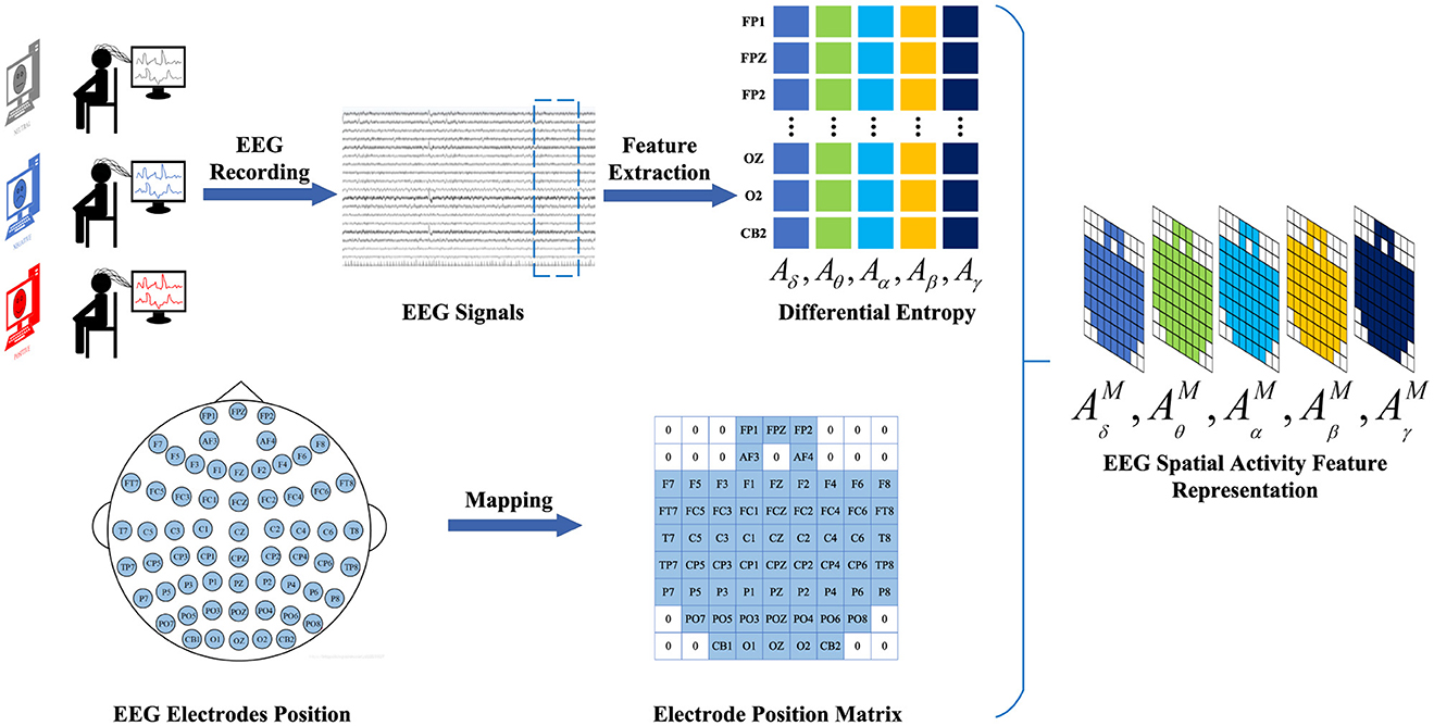
Figure 2. The construction process of EEG spatial activity feature representation. We adopt a time-frequency feature extraction method to extract 4-s EEG signal DE features from EEG signal samples. Subsequently, based on the electrode positions of the brain, the selected data are mapped onto the brain electrode position matrix. Finally, the electrode position matrices corresponding to different frequencies are superimposed to generate a spatial activity feature representation of the EEG signal.

2.2.2 EEG spatial topological ferture representation

To construct the EEG spatial topological feature representation, we employ the temporal-frequency feature extraction method to derive the DE of five frequency bands from all EEG channels across EEG signal samples within 4-s segments. We denote AB=(Aδ,Aθ,Aα,Aβ,Aγ)∈ℝNe×B as a frequency feature matrix comprising frequency bands extracted from the DE feature, where B ∈ represents the frequency band and Ne ∈ denotes the electrode. Subsequently, the frequency domain brain electrode network is defined as a graph G = (V, E, A), where V represents the set of vertices, with each vertex representing an electrode in the brain; E denotes the set of edges, indicating the connections between vertices; and A denotes the adjacency matrix of the brain electrode network G. Finally, the frequency-domain brain electrode position graph corresponding to different frequencies is overlaid to generate the spatial-frequency feature representation of EEG signals. Thus, the construction of the EEG feature representation AG=(AδG,AθG,AαG,AβG,AγG) is completed. The construction process of EEG spatial topological feature representation is illustrated in Figure 3.

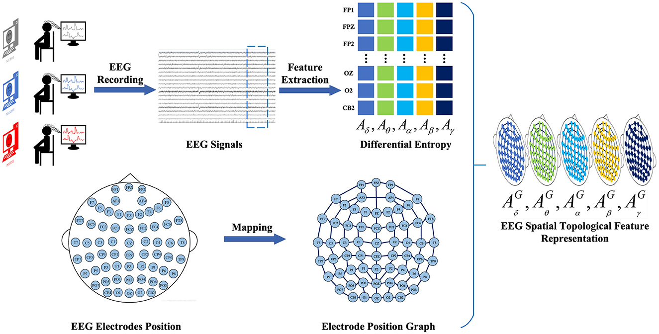
Figure 3. The construction process of EEG spatial topological feature representation. We employ a time-frequency feature extraction method to extract 4-s EEG signal DE features from EEG signal samples. Subsequently, the brain electrode position network is defined as a graph representation. Finally, the graph representations of electrode positions corresponding to different frequencies are superimposed to generate a spatial topological feature representation of the EEG signal.

2.3 Spatial feature perception extractor

Using EEG spatial activity features and EEG spatial topological features as inputs, a dual-branch spatial-activity-topological feature extractor module named SATFEM is designed. SATFEM can simultaneously extract spatial activity features and spatial topological features. The features extracted from the dual branches are fused at the feature fusion layer. Algorithm 1 shows the pseudocode for SATFEM. The SATFEM feature extractor consists of three main components: the spatial-topological feature extractor, the spatial activity feature extractor, and the feature fusion layer.

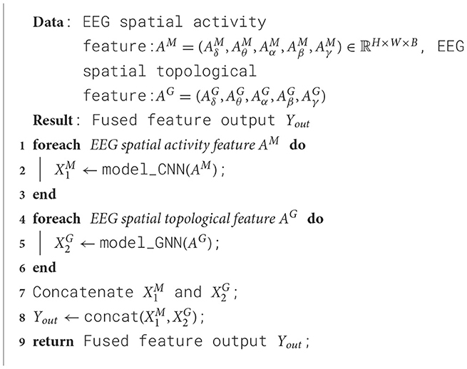
Algorithm 1. SATFEM.

2.3.1 Spatial topological feature extractor

The Graph Attention Network (GAT) is proposed to address issues in deep GNN models, such as inefficient information propagation and unclear relationships between nodes (Velickovic et al., 2017). GAT utilizes attention mechanisms to dynamically allocate weights between nodes, thereby enhancing the influence of important nodes and improving the efficiency of information propagation and clarity of relationships between nodes. Therefore, it is suitable for extracting EEG spatial topological feature representation as a feature extractor. This helps capture relationships between different functional areas in EEG feature representation, facilitating more accurate identification of different EEG signals. The input of GAT is the EEG spatial topological feature representation AG=(AδG,AθG,AαG,AβG,AγG).

In graph, let any node vi in the l − th layer correspond to the feature vector hi, where hi∈ℝd(l), and d(l) represents the feature dimension of the node. After an aggregation operation centered around the attention mechanism, the output is the new feature vector hi′, where hi′∈ℝd(l+1), and d(l+1) represents the length of the output feature vector. This aggregation operation is called the Graph Attention Layer(GAL).

Assuming the central node is vi, let the weight coefficient from neighboring node vj to vi be denoted as Equation 1.

eij=α(Whi,Whj),    (1)

The weight parameter W ∈ ℝd(l+1)×d(l) is used for the feature transformation of nodes in this layer. α(·) is the function used to compute the correlation between two nodes. The fully connected layer for a single layer is described as Equation 2.

eij=LeakyReLU(αT[Whi∥Whj]),    (2)

where the weight parameter α ∈ ℝ2d(l+1), and the activation function is designed as the LeakyReLU function. To better distribute weights, it is necessary to uniformly normalize the relevance computed with all leaders, specifically through softmax normalization as shown in Equation 3.

αij=softmaxj(eij)=exp(eij)∑vk∈Ñ(vi)exp(eik),    (3)

The weight coefficient α is calculated such that Equation 3 ensures that the sum of the weight coefficients for all neighbors is equal to 1. The complete formula for calculating the weight coefficients is described in Equation 4.

αij=exp(LeakyReLU(αT[Whi∥Whj]))∑vk∈Ñ(vi)exp(LeakyReLU(αT[Whi∥Whk])),    (4)

Following the calculation of the weight coefficients as described above, according to the weighted sum with attention mechanism, the new feature vector of node vi is obtained as shown in Equation 5.

hi′=σ(∑vj∈Ñ(vi)αijWhj),    (5) 2.3.2 Spatial activity feature extractor

The Residual Network (ResNet) is proposed to address the problem of degradation in deep CNN models. ResNet utilizes residual connections to link different convolutional layers, thereby enabling the propagation of shallow feature information to the deeper layers. Therefore, it is suitable for extracting EEG spatial Activity feature representation as a feature extractor.

The input of ResNet is the EEG spatial Activity feature representation AM=(AδM,AθM,AαM,AβM,AγM)∈ℝH×W×B. The EEG spatial Activity feature representation first goes through conv1, which consists of a 7 × 7 convolutional layer, a max pooling operation, and Batch Normalization. The conv1 layer is responsible for the initial processing of spatial information extraction and feature representation for EEG spatial Activity feature representation. Specifically, the input of conv1 is the spatial-frequency feature representation AM=(AδM,AθM,AαM,AβM,AγM)∈ℝH×W×B, where the shape of the spatial Activity feature representation is H × W × C, with H representing the height, W representing the width, and C representing the number of channels. Due to the number of frequency bands being 5, C = 5. However, this does not meet the input requirements of the original ResNet model, as the first convolutional layer in the original ResNet model requires an input channel size of 3. If the original model is used directly to process data with 5 input channels, channel conversion or padding operations are required, which may result in the loss of important information from the original data. Therefore, we replaced the first half of the ResNet model with a new convolutional layer that has 5 input channels, 64 output channels, a kernel size of 7 × 7, a stride of 2, a padding of 4, and no bias. The equations for conv1 of ResNet are shown in equations Equation 6.

C1=MaxPool(ReLU(BN(Conv7×7(AM)))),    (6)

where AM is the input of conv1 in the CNN branch, C1 is the output of conv1 in the CNN branch. Conv7 × 7(·) represents the convolutional layer operation with an output channel of 64, kernel size of 7 × 7, the stride of 2, and padding of 4. BN(·) represents the batch normalization layer operation, which performs batch normalization on the output of the convolutional layer. ReLU(·) represents the ReLU activation function, which applies the ReLU activation function to the output of the batch normalization layer. MaxPool(·) represents the max pooling layer operation, which performs max pooling using a 3 × 3 pooling kernel, a stride of 2, and padding of 1.

The features output from conv1 are processed through conv2x, conv3x, conv4x, and conv5x, respectively. Each of conv2x, conv3x, conv4x, and conv5x consists of 2 BasicBlocks. In BasicBlock, the input feature is added to the main branch output feature via a shortcut connection before being passed through a ReLU activation function. The equation of the main branch, as shown in Equation 7.

Xmain=BN(Conv3×3(ReLU(BN(Conv3×3(XBasicIN))))),    (7)

where XBasicIN is the input of BasicBlock, Xmain is the output of the main branch in the BasicBlock. Conv3×3(·) represents the convolutional layer operation with a kernel size of 3 × 3, the stride of 1, and padding of 1. BN(·) represents the batch normalization layer operation, which performs batch normalization on the output of the convolutional layer. ReLU(·) represents the ReLU activation function, which applies the ReLU activation function to the output of the batch normalization layer.

The shortcut connection allows the gradient to flow directly through the network, bypassing the convolutional layers in the main branch, which helps to prevent the vanishing gradient problem. The equation of the shortcut connection, as shown in Equation 8.

Xshortcut==BN(Conv1×1(Conv3×3(XBasicIN))),    (8)

where XBasicIN is the input of BasicBlock, Xshortcut is the output of the shortcut connection in the BasicBlock. Conv3×3(·) represents the convolutional layer operation with a kernel size of 3 × 3, the stride of 1, and padding of 1. Conv1 × 1(·) represents the convolutional layer operation with a kernel size of 1 × 1. BN(·) represents the batch normalization layer operation. ReLU(·) represents the ReLU activation function.

The addition of the input feature to the main branch output feature allows the network to learn residual mappings, which can be easier to optimize during training. The equation of the addition, as shown in Equation 8.

XBasicOUT=ReLU(Xmain+Xshortcut),    (9)

where Xmain is the output of the main branch, Xshortcut is the output of the shortcut connection, and XBasicOUT is the output of the BasicBlock. ReLU(·) represents the ReLU activation function.

2.3.3 Feature fusion layer

Utilizing EEG spatial activity feature representation and EEG spatial topological feature representation, the EEG spatial activity extractor and EEG spatial topological feature extractor respectively extract local features of EEG signals and functional connectivity of brain regions from EEG signals. Subsequently, the extracted EEG spatial activity feature representation information and EEG spatial topological feature representation information are fused in the Feature Fusion layer, as outlined in Equation 10. The fused dual-branch network module is referred to as the spatial-activity-topology feature extraction network module, abbreviated as SATFEM.

Yout=Fusion(X1M∥