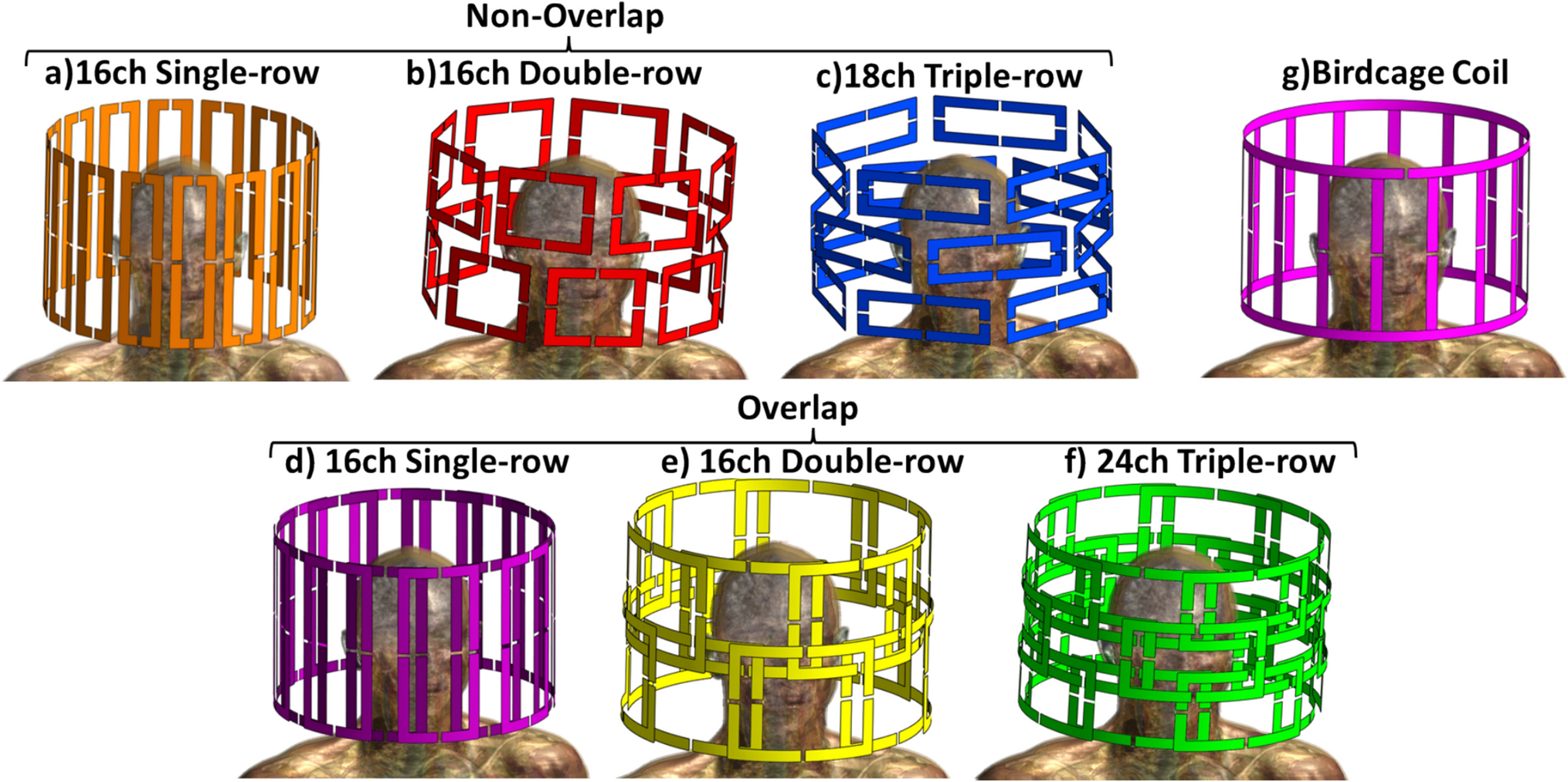
MR measurements were performed on a Magnetom 9.4T Plus MRI scanner (Siemens Healthineers, Erlangen, Germany) running Syngo VE12U software, equipped with a 16-channel pTx system (1kW RF power per channel) and a SC72 whole-body gradient system. A custom-built head array coil (16 transmit, 31 receive elements) was used [14]. The system was operated assuming the following hardware limitations: maximum RF magnitude: 185 V per channel; maximum gradient magnitude: 65 mT/m; maximum gradient slew rate: 185 T/m/s. Data was acquired from 14 healthy adults (age: 24...54 years, 9 male, 5 female). All experiments were performed with approval of the local ethics committee. Before each MR-experiment, informed signed consent was obtained from each volunteer.

1. Toolbox design and usage

For using the FastPtx toolbox, multiple steps are necessary as of now. All those steps are outlined here and will be explained in more detail in the following chapters.

Since pulse calculation relies on \(B_1^+\) and \(B_0\) maps, those need to be acquired. After reconstruction, they have to be stored in a MATLAB file, together with a binary mask of the region of interest, in our case a brain mask. \(B_1^+\) fields have to be provided in [nT/V] and \(B_0\) maps in [\(\Delta\)Hz]. The FastPtx toolbox is then executed by running a short python script, in which system limits, desired FA distribution and the desired number of iterations for optimization, as well as one or multiple files with \(B_1^+\)/\(B_0\) maps are specified. The resulting optimized RF and gradient waveforms will be returned as PyTorch arrays by the FastPtx toolbox. They can either be used in custom code or passed onto another function of the FastPtx toolbox, which will write the pulse into a .ini file as required by the Siemens VE12U system we used. This file can then be transferred to the MRI scanner, for example via the local network.

The toolbox consists of three main modules. One module is called io.py and handles data in- and output. It includes functions for reading \(B_1^+\) maps,\(B_0\) maps, and VOP files, as well as functions to read and write pTx pulses in the .ini format required by the scanner. The second module, smallTipAngle.py, consists of a class that has methods for forward simulation, the cost function, and the optimization code. The third module, bloch.py, contains a class which is derived from smallTipAngle.py and overwrites the forward simulation methods. By doing so, most steps only needed to be implemented once even though both STA and Bloch simulation are supported.

2. Generation of \(B_1^+\) maps

Individual-channel \(B_1^+\) maps and a \(B_0\) map of each subject were recorded with a centric-reordered 3D saturated single-shot turboFlash (3DsatTFL) sequence [15, 16]. A sinc pulse with a duration of 5 ms and a bandwidth of 4000Hz was used for saturation. RF interferometry [17] was used by phase-shifting one Tx channel by 180° at a time. Recovery time \(T_\) between scans was 0.5 s for the relative \(B_1^+\) scans and 7.5 s for all other scans. Other sequence parameters wereInterface: TR=2.44 ms, TE=0.75 ms, BW=700 Hz/Px, asymmetric echo, elliptical k-space filling, GRAPPA [18] 2x2, nominal flip angle(FA) excitation=2°, nominal FA presaturation=70°, \(\tau\)-excitation=200 µs, \(\tau\)-saturation=5000 µs, 795 k-space encoding steps, readout duration 1.94 s, matrix: 64\(\times\)64\(\times\)64, resolution 3.5 mm isotropic (\(\tau\) indicates the pulse duration). Acquisition time: 197 s. An additional repetition with a longer TE was included in the sequence, which allowed for the estimation of \(B_0\) maps. Based on the 3DsatTFL data, brain extraction was performed using a neural network [16].

3. RF pulse simulation

Software for pTx pulse optimization was developed in Python 3.9 using the PyTorch toolkit version 1.13.0. Local SAR supervision was performed using a Virtual Observation Points (VOP) model [19] with 208 VOPs, which was specifically generated for the RF coil in use. For VOP generation two voxel models (Duke and Ella, virtual family [20]) were simulated using CST Microwave Studio. VOP compression was performed using the compression algorithm by Orzada et al. [21]. The worst-case overestimation factor of the resulting VOPs was 8.4%.

Fig. 1

Optimization result of a non-selective 10° pTx pulse with a duration of 520 µs. The optimization took 66 s. Subplot (a) displays the simulated FA and the resulting phase. Subplot (b) shows the magnitude and phase of all RF waveforms. The gradient waveforms and the corresponding slew rates and k-space trajectories can be seen in subplot (c). If appropriate information such as sequence timing and target FA distribution is given, SAR and RMSE can be calculated and displayed (subplot (d))

Fig. 2

Simulated flip angle (FA) distribution in a subject that was not part of the UP pulse design database. a: CP mode rectangular pulse as calculated by the MR scanner. b: CP mode rectangular pulse scaled to a mean FA of 10°. c: Tailored non-selective pulse for this specific subject. d: Universal non-selective pulse. The CP mode pulse excites with a wide FA distribution. Additionally, the MR scanner scales RF power too low, so that the median FA is significantly lower than the target FA of 10°. Both pTx pulses excite with an appropriate median FA. As expected, the tailored pulse outperforms the universal pulse with regard to FA homogeneity

A full Bloch simulation, taking into account previously recorded \(B_1^+\) and \(B_0\) maps, was implemented. It allows for accurate simulation of arbitrary RF and gradient pulses. Additionally, to allow for expedited simulation of small tip angle pulses, a simulation based on the small tip angle approximation was also implemented. It follows the forward simulation of the spatial domain method [1], in which gradient waveforms, \(B_0\) map and \(B_1^+\) sensitivities are assembled into a system matrix (see Equation 3).

Using single-channel \(B_1^+\) maps and a \(B_0\) map of one or several subjects, the resulting FA distribution of a pTx RF pulse with underlying gradient pulse can be simulated using both methods. With consideration of the average repetition time of the RF pulses, their maximum local SAR can be calculated.

4. RF pulse optimization

All optimizations were run on a dedicated server for data reconstruction and pulse optimization which was equipped with a NVIDIA RTX A6000 GPU with 48 GiB of memory and a AMD Ryzen Threadripper PRO 3995WX 64-Core CPU. All optimizations were performed on the GPU unless stated otherwise. Optimization of RF and gradient waveforms was performed using the AdamW algorithm [22]. As it employs a gradient descent based method, the optimization greatly benefits from the autodifferentiation capabilities of PyTorch. The learning rate was set to \(4\cdot 10^\) and the internal momentum parameters of the optimizer were reinitialized after every set of 1000 iterations, using the former best performing pulse as start value. Each sample and each channel of the RF and gradient waveforms was optimized freely, resulting in a very large number of parameters that needed to be optimized.

To respect hardware- and regulatory limits, a cost function was designed. It uses carefully chosen weights to balance different metrics, which were determined experimentally.

$$\begin \begin c(p,g) =\,&pen_\text (g,p) + err_\text (p) + err_\text (g) + err_\text (g) + err_\text (p,g) \\ +&pen_\text (p) + pen_\text (g) + err_\text (p) \end \end$$

(4)

All elements of the cost function depend on the gradients g, the RF-pulse p or both. It consists of penalty terms (named \(pen_\)), which have a relatively low magnitude that is usually positive non-zero and scales with the input, and of error terms (named \(err_\)) which have a value of zero until a certain limit is exceeded. The exact equations for all terms are listed in Table 1. By defining a target flip angle distribution, a pulse duration, and a sampling interval, pTx pulses can be optimized using either the small tip angle approximation or the Bloch simulation.

Based on the \(B_1^+\) and \(B_0\) maps of the first 9 subjects, a universal pulse (UP) with a nominal flip angle of 10° and a SAR limit of 2.3 W/kg at a TR of 19.7 ms was designed. Pulse duration was 520 µs with a raster time of 10 µs. Optimization of all three gradient axes and 16 complex RF waveforms (in total 1820 real-valued parameters) was run on the small tip angle model for 7,500 iterations. Subsequently, the RF waveforms were refined by 2,500 steps of optimization based on the Bloch model, using the RF and gradient waveforms of the STA optimization as a starting point. By designing the pulse for 10°  it was possible to scale it down to the required flip angle without risk of exceeding SAR or power limits. Following the small tip angle approximation, the pulse flip angle could be scaled linearly by scaling the pulse voltage. This allowed a single universal pulse to be designed and used for different applications requiring different small flip angles, making the pulse even more universal.

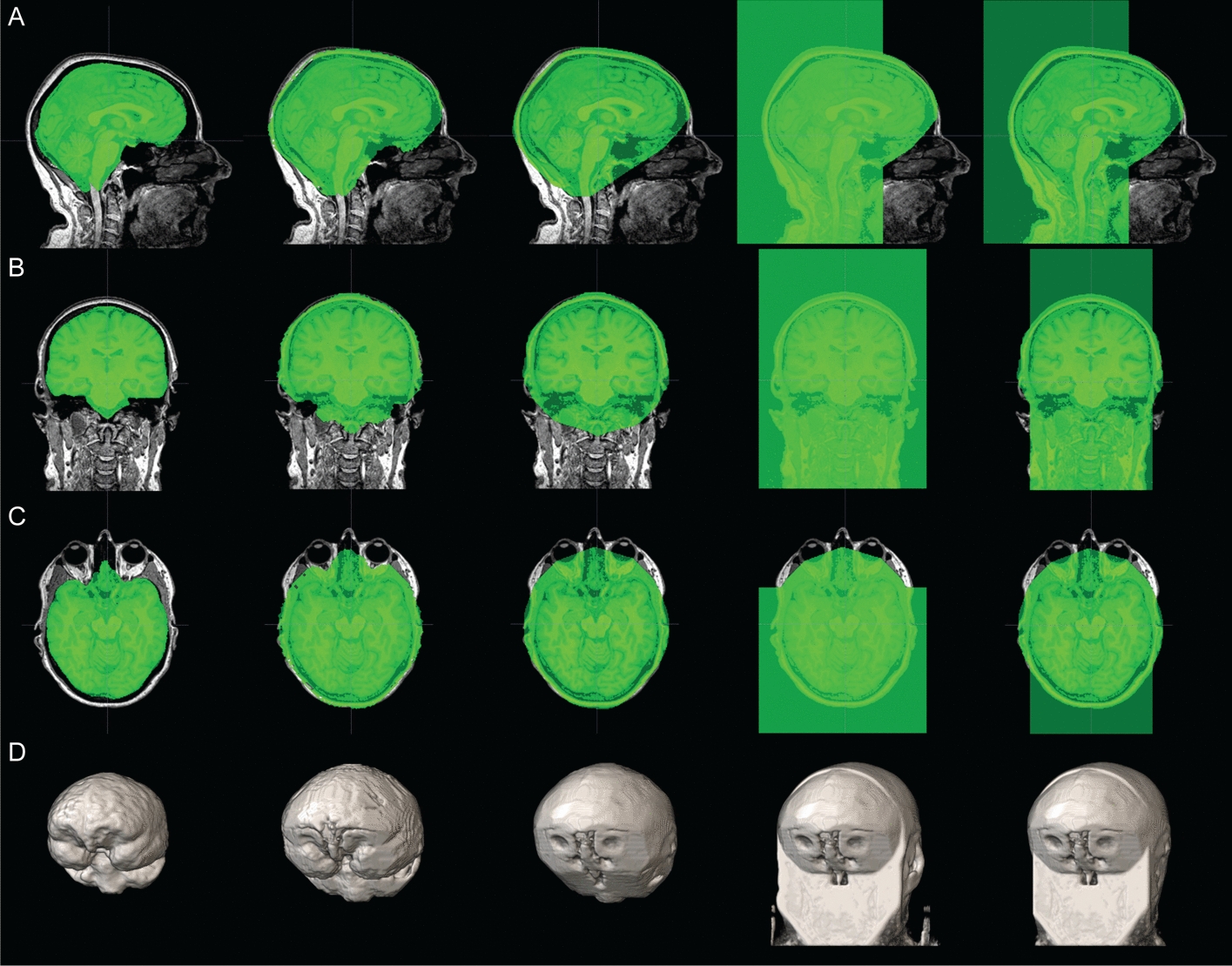
Fig. 3

Sagittal view of MPRAGE brain images of 5 different subjects. The first row (“CP”) shows images using a rectangular CP mode pulse for excitation. In the second row (“TP”) a non-selective subject-specific tailored excitation pulse was used. In the third row (“UP”) excitation was done with a non-selective universal pulse which was designed on 9 subjects. CP mode excitation creates severe image inhomogeneities, e.g., near the cerebellum. This is greatly reduced in the images acquired with either of the pTx pulses. None of the subjects displayed here was part of the UP design database

Fig. 4

Coronal view of MPRAGE brain images of 5 different subjects. The first row (“CP”) shows images using a rectangular CP mode pulse for excitation. In the second row (“TP”) a non-selective subject-specific tailored excitation pulse was used. In the third row (“UP”) excitation was done with a non-selective universal pulse which was designed on 9 subjects. CP mode excitation creates severe image inhomogeneities, e.g., near the cerebellum. This is greatly reduced in the images acquired with either of the pTx pulses. None of the subjects displayed here was part of the UP design database

Fig. 5

Saggital view of GRE brain images of 5 different subjects. The same excitation pulses as for the MPRAGE sequence (Figs. 2 and 3) were used, scaled to 5° flip angle. Similar inhomogeneities near the cerebellum can be observed for the CP mode pulses, while both pTx pulses improved homogeneity

For five additional subjects that were not part of the UP design database, a TP was designed using the same design criteria. In this case, however, optimization was performed on the small tip angle model only to keep computation time short and stopped after 2,500 iterations. For both pulses, Bloch simulation was used to evaluate the pulses’ performance.

Furthermore, to test the toolbox’s performance in the high-FA-regime, a 90° pulse was designed. This was done by first designing a 9° pulse using the STA, under appropriately scaled peak power constraints, for 3500 iterations. The RF waveforms were then scaled up by a factor of 10 and refined with 1000 iterations of the Bloch simulation, optimizing the RF waveforms only. This pulse was designed without SAR constraint since it was only played out once, as preparation pulse for a satTFL sequence.

As a benchmark for the free waveform tailored pulse calculated with FastPtx, a 3 kT point pulse was generated for a single subject. The optimization was performed similarly to the spatial domain method [1] using the variable exchange method [3] to solve the magnitude-least-squares problem with 20 iterations on an unregularized minimization. The k-space location of the first two kT points was chosen by randomly generating 5,000 pairs of k-space positions in the range \(-14\,m^ \le k_ \le 14\,m^\) and selecting the one that gave the best performance for the given scenario. The third kT point was positioned in the center of the k-space. The three sub pulses were designed to be 130 µs long with a pause of 60 µs between sub pulses for gradient blips.

5. MPRAGE measurements

A 3D MPRAGE protocol was set up with the following parameters: TR1=3,360 ms, TR2=6.16 ms, TE=3.03 ms, BW=420 Hz/px, matrix size=264x264x224, resolution=0.8 mm isotropic, GRAPPA 2x2, Inversion Time=1,340 ms, FA=9°. The voltage of the adiabatic inversion pulse (HS4, 12.8ms) was scaled to 460V, so that it attributed to \(\approx\)7 W/kg of local SAR.

For excitation, three different pulses were used. The first protocol (MPRAGECP) used a conventional rectangular pulse in CP mode. For the second protocol (MPRAGEUP), the universal pulse was scaled down to 9° and used as excitation pulse. The third protocol (MPRAGETP) used the subject-specific, tailored pTx pulse which was also scaled down to 9°. All three protocols used the adiabatic HS4 pulse for inversion.

All three excitation pulses were applied on 5 subjects which were not in the design database of the universal pulse and results were compared.

6. GRE measurements

To obtain images with a T2* weighted contrast, 3D GRE images with the following parameters were acquired: TR=11 ms, TE=7 ms, BW=260 Hz/px, matrix size=264x264x224, resolution=0.8 mm isotropic, GRAPPA 2x2, FA=5°.

The excitation pulse was varied similarly as for the MPRAGE sequence: The first protocol (GRECP) used a conventional rectangular pulse, second protocol (GREUP) the universal pulse scaled down to 5°, and the third protocol (GRETP) used the subject-specific, tailored pTx pulse which was also scaled down to 5°. All three pulses were applied on the same 5 subjects which were not in the design database of the universal pulse.

7. Simulation experiment

In a simulation-only experiment on a single-subject dataset, the CP mode pulse used for the MPRAGE sequence was scaled to a mean FA of 10°, which resulted in 0.92 W/kg of local SAR. Using this as a SAR constraint for optimization, a pTx pulse was designed with the goal of outperforming the CP mode pulse while maintaining the same SAR budget. Optimization parameters were comparable to those for the tailored pulses on single subjects.

8. Slab selective excitation

A slab-selective pulse (thickness 50 mm, orientation transversal\(\rightarrow\) coronal 45°, FA 10°) was designed starting from a conventional CP mode sinc pulse with a trapezoidal slice-selection gradient. Parameters were: time-bandwidth product 8, pulse duration 1.2 ms, total duration (including gradients) 2.4 ms. The pulse was used as a starting point for free optimization of ptx RF and gradient waveforms with the goal of FA homogenization. A universal pTx pulse was designed using the same design database as before. Optimization was run for 20,000 iterations.

Fig. 6

A 90° rectangular CP mode pulse scaled by the MRI system (a) and scaled up to an average FA of 90°(b), compared to a 90° tailored pTx pulse (TP, c), both measured using a satTFL sequence. The right column (c) shows the simulated FA distribution of the 90° TP. Anatomic features are visible in all three maps, which is likely to be an artifact from the utilized \(B_1^+\) mapping sequence

Fig. 7

Simulated flip angle (FA) distribution of a slab selective pulse in a subject that was not part of the UP pulse design database. a: CP mode sinc pulse as calculated by the MR scanner. b: Universal pTx pulse. The CP mode pulse excites with a wide FA distribution. Additionally, the MR scanner scales RF power too low, so that the median FA is significantly lower than the target FA of 10°. The universal pulse excites more homogeneously with the mean FA closer to the target than in the sinc pulse

Fig. 8

GRE images recorded with slab selective pulses. a: CP mode sinc pulse. b: optimized pTx UP. While both pulses achieve a clean slice profile, excitation in the cerebellum is more homogeneous with the pTx pulse

The so designed pulse was then applied on a subject which was not part of the design database. The same 3D GRE sequence was used as for non-selective excitation. This allowed not only to observe the excited area, but also to get an impression of the slice profile since the entire brain was encoded in the resulting image. FA distribution and image were compared to the sinc pulse.

9. Robustness of pulses

A potential source of error in pTx excitation is a lack of stability in the transmit path of the MR scanner. To investigate the effect of slightly imprecise Tx channels, a simulation experiment was performed. A magnitude factor and a phase offset were generated for each channel. These parameters were drawn from a Gaussian normal distribution with a standard deviation of 5% for the amplitude and 5° for the phase. These values were chosen because they are similar to the accuracies the scanner manufacturer specifies for SAR supervision measurements (12% power, 5° phase on 7 tesla systems), implying that these are the maximum deviations to be expected when playing out RF pulses. The UP and CP mode pulse were then adjusted by these values and simulated on \(B_1^+\) maps from a subject who was not part of the UP design database. To get a wide range of magnitude and phase error combinations, this experiment was repeated 10 times.

While this issue is not related to our toolbox but instead affects all applications, it is important to get an understanding of the scale of the effects caused by those imprecisions. In contrast to the extensive experience with conventional pulse shapes, there is little experience with freely designed RF waveforms and their stability, so this simulation experiment can give an estimate of the impact of instabilities on the pulses generated by FastPtx.